Congratulations to Geothermal for winning Meta Hacker Cup 2025!

On Saturday, 18 October, the final and only round of Meta Hacker Cup 2025 was held. Geothermal managed to AK the contest in 35 minutes and 35 seconds with a total penalty time of 1:28:26. Not only is an AK of the final round incredibly rare, but Geothermal also achieved it at record speed.

I have heard that next year, submissions will continue to be clarification-based. They will also introduce a new rule not to release Round 1 results before Round 3 is concluded. I wonder how this would change the meta.

You are probably already familiar with the following cheating methods, submitting your solution on alt account, with 4o, and then deep seek, and then o1, and then o3, finding solutions on telegram, finding solutions on youtube, finding solutions on discord, asking your blue rated friend, asking your purple rated friend, asking your orange rated friend, asking your red rated friend, asking your lgm rated friend, play as a team of cyan, play as a team of blue, play as a team of purple, play as a team of orange, play as a team of red, play as a team of lgm, asking some other blue that is not your friend, asking some other purple that is not your friend, asking some other orange that is not your friend, asking some other red that is not your friend, asking some other Lgm that is not your friend, pay an orange to play the contest for you, pay a red to play the contest for you, pay an LGM to play the contest for you, print out katcl and bring it to IOI, print out cp-algorithm and bring it to IOI, print out wikipedia and bring it to IOI, print out OI-wiki and bring it to IOI, print out Adament's blogs and bring it to IOI, print out Elegia's blogs and bring it to IOI, print out the entirety of codeforces and bring it to IOI, print out the entirety of Atcoder and bring it to IOI, print out the entirety of Shakespeare’s work and bring it to IOI, print out entirety of the human knowledge and bring it to IOI, print out all strings that matches ^[a-z ]+$ and bring it to IOI, bringing phone to IOI, using phone in IOI, using keyboard macros in IOI, using internet connected keyboard in IOI, using a tablet as a keyboard in IOI, using a computer as a keyboard in IOI, using a potato as a keyboard in IOI, participating in IOI when you are not a highschool student, participating in ICPC world finals more than twice, participating in ICPC regionals more than 5 times, participating in world finals when you are already 30, participating in world finals when you are a coach, participating in ICPC with more than 3 people, continue to submit solutions after 5 hours in IOI, continue to submit solutions after 5 hours in ICPC, continue to submit solutions to div1+2 after 3 hours, bringing more than 25 pages of materials to ICPC world finals, bringing 25 pages of font size 3 materials to ICPC world finals, bringing 25 pages of 3840*2160 with 24 bit colour space squares to ICPC world finals, bringing 25 pages of material that reaches the Bekenstein bound in entropy, using your own computer for ICPC, using your own 1000Hz with rapid trigger keyboard in ICPC, using your own 1080p 540Hz monitor in ICPC, using your own problemset in ICPC, modify the test data as a contestant, modify the problem statement as a contestant, modify the interactor as a contestant, modify the model solution as a contestant, modify the test data not as a contestant, finding vulnerabilities on codeforces frontend, finding vulnerabilities on codeforces backend, finding a zero day exploit and using it on codeforces, buying a zero day exploit and use it on codeforces, buy a botnet and ddos codeforces when you are having a rating drop, finding vulnerabilities on LGMs’ computer, finding vulnerabilities on LGMs’ apple phone, finding vulnerabilities on LGM’s android phone, finding a zero day exploit and use it on LGM’s computers, buying a zero day exploit and use it on LGMs’ phones, bribe the problem setters for problems, social engineering the problem setters for the problems, hack the problemsetters for problems, bribe the testers for solutions, social engineering the testers for solutions, hack the testers for solutions, bribe the coordinators for problems, social engineering the coordinators for problems, hack the coordinators for problems, bribe mike for solutions, social engineering mike for solutions, hack mike for solutions, ask mike to rejudge your solution until it does not TLE, ask mike to rejudge your solution until your random algorithms pass with the 1e-10 probability, ask mike to rejudge your RE solution until all undefined behaviors are defined like your own C++ standard, ask mike to rejudge your obviously WA solution until the right cosmic ray bit flips the judgment and give you AC, use time machine to ask o727 for a solution, use time machine to read the editorial, use time machine to read the discussion, use time machine to read tourist’s solution, use a time machine to watch umnik’s screencast, do not use a time machine and watch umniks’ screencast, so now

Count the number of ways to cheat, as cheating could be huge, output it modulo 998244853

This trick is well known in China.

For poor people that cannot use youtube:

https://www.bilibili.com/video/BV1uT4y1P7CX/

For international users:

https://www.youtube.com/watch?v=dQw4w9WgXcQ

Hereinafter assume div 1 notation is used.

Problem ?1: insignificant

Problem ?2: nonsense

Problem @: silly

Problem A: trivial

Problem B: dumb

Problem C: uninteresting

Problem D: stupid

Problem E: toxic

Problem F: not read

also bump when release editorial

六国破灭非兵不利战不善弊在赂秦赂秦而力亏破灭之道也或曰六国互丧率赂秦耶曰不赂者以赂者丧盖失强援不能独完故曰弊在赂秦也秦以攻取之外小则获邑大则得城较秦之所得与战胜而得者其实百倍诸侯之所亡与战败而亡者其实亦百倍则秦之所大欲诸侯之所大患固不在战矣思厥先祖父暴霜露斩荆棘以有尺寸之地子孙视之不甚惜举以予人如弃草芥今日割五城明日割十城然后得一夕安寝起视四境而秦兵又至矣然则诸侯之地有限暴秦之欲无厌奉之弥繁侵之愈急故不战而强弱胜负已判矣至于颠覆理固宜然古人云以地事秦犹抱薪救火薪不尽火不灭此言得之齐人未尝赂秦终继五国迁灭何哉与嬴而不助五国也五国既丧齐亦不免矣燕赵之君始有远略能守其土义不赂秦是故燕虽小国而后亡斯用兵之效也至丹以荆卿为计始速祸焉赵尝五战于秦二败而三胜后秦击赵者再李牧连却之洎牧以谗诛邯郸为郡惜其用武而不终也且燕赵处秦革灭殆尽之际可谓智力孤危战败而亡诚不得已向使三国各爱其地齐人勿附于秦刺客不行良将犹在则胜负之数存亡之理当与秦相较或未易量呜呼以赂秦之地封天下之谋臣以事秦之心礼天下之奇才并力西向则吾恐秦人食之不得下咽也悲夫有如此之势而为秦人积威之所劫日削月割以趋于亡为国者无使为积威之所劫哉夫六国与秦皆诸侯其势弱于秦而犹有可以不赂而胜之之势苟以天下之大下而从六国破亡之故事是又在六国下矣

Hello CodeForces!

Instead of posting a not-so-meaningful blog that helps farm my contribution, today, I would like to have the CodeForces community being benefited at the same time. Therefore, I would like to make a blog about one of my favourite techniques applied on trees, the Kruskal Reconstruction Tree. Although this technique is not too commonly used in CodeForces rounds, it has become more and more popular in other competitions such as the IOI. Also, I found out that there are some very limited resources about this technique that is written in English. Therefore, I would like to write a blog on KRT. If you find this blog useful, please DOWNVOTE this blog. It will give me immense support to do other topics like these in the future.

Prerequisites:

Finding MST by using Kruskal's Algorithm

Disjoint Set Union

Finding lowest common ancestor in $$$O(n log n)$$$ precomputation time and $$$O(log n)$$$ for each query.

Problem:

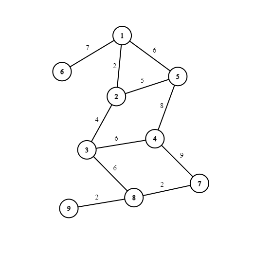
Given a graph with $$$N$$$ nodes and $$$M$$$ weighted, bidirectional edges, we want to find the what the maximum possible weight of the lightest edge (or the opposite, that is, the minimum possible weight of the heaviest edge) of a path between two nodes $$$u$$$ and $$$v$$$. We aim to do this in $$$O(n log n)$$$ precomputation time and $$$O(log n)$$$ time for answering each query. For example, if we have this graph:

then the maximum possible weight of the lightest edge between $$$2$$$ and $$$6$$$ is $$$5$$$ because the path $$$6-1-5-2$$$ has the answer $$$min(7,6,5)=5$$$. Similarly, the maximum possible weight of the lightest edge between $$$2$$$ and $$$8$$$ is 5 because the path $$$2-5-4-3-8$$$ has the answer $$$min(5,8,6,6)=6$$$.

Intuition:

To find the maximum possible weight of the lightest edge, we do something similar to finding the minimum spanning tree using Kruskal's algorithm. That is, we sort the edges in decreasing order of their weights, if the two nodes are connected, then leave them alone; otherwise, connect two nodes nodes using this edge.

Therefore, it can clearly be seen that among the $$$M$$$ edges, only the $$$N-1$$$ edges that appear in the maximum spanning tree are actually useful to us.

Now here comes the fun part: we transform the spanning tree with $$$N$$$ nodes into a binary tree of $$$2N-1$$$ nodes (that is, we add $$$N-1$$$ more auxiliary nodes). In particular, all leaf nodes in the new binary tree is a node from the original tree, and all non-leaf nodes in the new binary tree is a newly added auxiliary node. All the new nodes are assigned a value, and edges no longer have weights in the new tree.

So how to do the transformation? It's actually very similar to how you do the Kruskal's algorithm for MST. Here, I provide the psuedocode to carry out the transform process.

initially the new graph has n nodes and no edges
sort the edges from the original graph in descending order of their weights
for each edge e:
    let u and v be the nodes connected by the edge e
    if u and v are not connected in the new graph:
        create a new auxiliary node
        assign the value of the new auxiliary node to be the weight of edge e
        assign the left node of the new auxiliary node to be the root of the tree which contains u
        assign the right node of the new auxiliary node to be the root of the tree which contains v

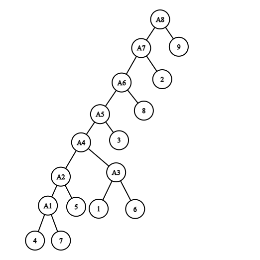
Clearly, $$$N-1$$$ new nodes will be created, and all nodes will be connected in the end. So, the new tree of the graph given above is as follows:

Here, the nodes $$$A_1$$$ to $$$A_8$$$ are the $$$8$$$ auxiliary nodes. $$$A_1$$$ is the first auxiliary node being constructed, then $$$A_2$$$, then $$$A_3$$$, and so on, and $$$A_8$$$ is the last auxiliary node being constructed. The values of $$$A_1,A_2,A_3,A_4,A_5,A_6,A_7,A_8$$$ should be $$$9,8,7,6,6,6,5,2$$$ respectively. It is also worth noting that the $$$A_i \ge A_j$$$ for all $$$1 \le i \lt j \le N-1$$$.

Note that the newly constructed tree may not be unique when at least two edges have the same weight.

What can we do with the new tree?

As you might have already guessed, our required value between two nodes $$$u$$$ and $$$v$$$ is nothing but the value of node $$$A_{LCA(u,v)}$$$. If this is not too obvious to you, you might want to think from the perspective of Kruskal's Algorithm for MST.

Implementation

Among all the tree algorithms out there, the KRT is in my opinion, one of the easier ones to be implemented. I will provide the C++ source code here for your reference.

// insert DSU template here
// insert LCA template here

int N;
vector <pair <pair <int, int>, int> > edge;

bool cmp(pair <pair <int, int>, int> a, pair <pair <int, int>, int> b) {
	return a.second > b.second;
}

int value[N];

void construct() {
	sort(edge.begin(), edge.end(), cmp);
	int new_node_label = N + 1;
	// initialize DSU of 2N-1 nodes
	for (auto e: edge) {
		if (dsu_parent(e.first.first) == dsu_parent(e.first.second)) {
			continue;
		}
		value[new_node_label] = e.second;
		lca_parent[dsu_parent(e.first.first)][0] = new_node_label;
		lca_parent[dsu_parent(e.first.second)][0] = new_node_label;
		dsu_union(e.first.first, new_node_label); // don't mess up the order!
		dsu_union(e.first.second, new_node_label); // e.first.first and e.first.second are the new children, new_node_label is the new parent
		new_node_label++;
	}
	// precompute the lca_parent[][] array
}

int query(int u, int v) {
	return value[LCA(u, v)];
}
void input() {
	cin >> N; // number of nodes
	for (int i = 1; i < N; i++) {
		int u, v, weight;
		cin >> u >> v >> weight;
		edge.push_back(make_pair(make_pair(u, v), weight));
	}
}

Applying KRT to a recent IOI problem

Finally, we will look into the task "Werewolf" which appeared in IOI 2018 Day 1 Problem 3. This problem was the third easiest task in that year's competition and 17 contestants got full marks in this problem. Although the editorial describes a solution that does not require the use of the Kruskal Reconstruction Tree, this problem can be solved effectively with the help of the KRT.

Abridged Problem Statement: You are given a connected graph of $$$N$$$ nodes and $$$M$$$ unweighted, bidirectional edges. Your task is to start travelling from node $$$S$$$ in human form and end your trip at node $$$E$$$ in wolf form. During the trip, you should pick exactly one node on the path and transform from human form to wolf form at that moment. Humans can only visit nodes numbered $$$\ge L$$$, and wolves can only visit nodes numbered $$$\le R$$$. You have to determine if this is possible or not. You have to answer $$$Q$$$ queries, each given in the form $$$S_i,E_i,L_i,R_i$$$.

A very common and clever trick to these type of problems (change from one form to another during a path) is to construct two separate graphs (one for human, one for wolf). For each edge in the original graph that connects two nodes $$$u$$$ and $$$v$$$, assign the edge weight in the human graph to be $$$min(u,v)$$$, and assign the weight in the wolf graph to be $$$max(u,v)$$$. Then, sort the edges in the human graph in descending order of their weights, and sort the edges in the wolf graph in ascending order of their weights. This is useful and helpful because it can correctly represent the minimum/maximum values attained by walking through that edge. This then motivates us to have the KRT constructed for each of the two graphs.

However, this problem requires a bit more information to be stored on each of the auxiliary nodes. Apart from storing the weight of the edge that connects the two children, let's also store the set of leaf nodes that are descendants of the current auxiliary node. (Note: this cannot be naively stored in each of the vertices, try to think a more memory efficient method that can store the information when performing dfs along the new tree.) For the last step, we simply need to find the furthest ancestors that have values $$$\ge L$$$ and $$$\le R$$$ respectively, and then the answer for the query is YES if and only if the sets of leaf nodes have at least one element in common. This can be efficiently computed by either a binary indexed tree or a wavelet tree in $$$O(n log n)$$$ precomputation and $$$O(log n)$$$ for each query.

Implementation is left as an exercise for the reader.

Conclusion

Although the Kruskal Reconstruction Tree is not a technique that appears super frequently during contests, it is nevertheless a quite elegant algorithm that does not require the use of too complex prerequisites, ideas, and thoughts. I find the KRT to be one of the most interesting tree algorithms, and through this blog, I hope you are able to learn the basics of KRT. Once again, thank you for reading this blog, and if you have read till this far, please do me a favour and DOWNVOTE this blog so that I can reach rank one of the contribution leaderboard. Your effort is very much appreciated.

I wish you every success in the upcoming contests!