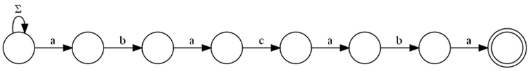
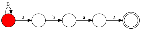
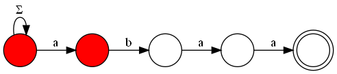
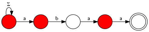
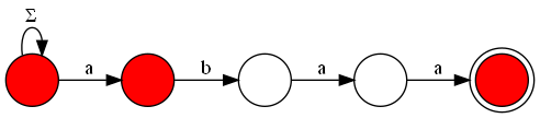
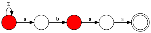
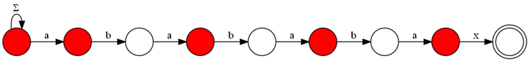
In this problem, we want to count the number of strings of length $$$n$$$ that have at least one occurrence of the given substring. To do this, we will use the Knuth-Morris-Pratt (KMP) algorithm and the automaton constructed from it, with a complexity of $$$O(m)$$$.

If $$$n$$$ were small, we could solve this problem using dynamic programming, calculating, for each $$$1 \leq i \leq n$$$, how many ways we can reach state $$$0 \leq j \leq m$$$ of the automaton (representing a string with the last $$$j$$$ characters equal to the first $$$j$$$ of $$$s$$$). This solution has $$$n \cdot m$$$ states with transitions of the size of the alphabet, resulting in a time complexity of $$$O(26 \cdot n \cdot m)$$$, which is too slow for this problem, since $$$n$$$ can go up to $$$10^{18}$$$.

Therefore, we need a faster way to solve this problem, which can be achieved by visualizing the KMP automaton as a graph. In this graph, we will have all the states of the automaton as nodes, and the transitions as edges. Additionally, to ensure that we do not count repeated strings or miss counting strings that do not end in the acceptance state (but have passed through this state at least once), we add a new node that will hold all strings that have passed through the acceptance state at least once. Thus, the acceptance state must have an edge to this final state, and to count all the possibilities of strings that have passed through this state once, the final state must have $$$26$$$ edges directed to itself, one for each letter of the alphabet.

Let $$$A$$$ be the adjacency matrix of the constructed graph. We know that $$$A^k$$$ will contain the number of paths of length $$$k$$$ between any two vertices. From this, we can observe that the answer to the problem will be the number of paths of length $$$n+1$$$ from the initial state of the automaton to our final state, since we must consider all letters used in the string and also the additional step between the acceptance state and the final state. We can calculate the matrix $$$A^{n+1}$$$ using the fast exponentiation algorithm with matrix multiplication, resulting in a final complexity of $$$O(m + m^3 \cdot \log(n))$$$, which is sufficient for the limits of this problem.

#include <bits/stdc++.h>
 
using namespace std;
 
typedef long long ll;
 
const int MAXM = 100;
 
int MOD = 998244353;
 
// exponenciacao de matrizes para contar o numero de caminhos no automato
 
struct Matrix {
    int r, c;
    vector<vector<int>> mat;
 
    Matrix(int n, int m, bool id = false): r(n), c(m), mat(r, vector<int>(c, 0)) {
        if (id) {
            for (int i = 0 ; i < min(r, c) ; i++)
                mat[i][i] = 1;
        }
    }
 
    Matrix operator*(const Matrix &o) {
        assert(c == o.r);
 
        Matrix result(r, o.c);
        for (int i = 0 ; i < r ; i++) {
            for (int j = 0 ; j < o.c ; j++) {
                ll sum = 0;
                for (int k = 0 ; k < c ; k++) 
                    sum = (sum + (1LL * mat[i][k] * o.mat[k][j])) % MOD;
                result.mat[i][j] = sum;
            }
        }
 
        return result;
    }
};
 
Matrix binpow(Matrix a, ll b) {
    Matrix res(a.r, a.c, true);
 
    while (b) {
        if (b&1) res = res * a;
 
        a = a * a;
        b >>= 1;
    }
 
    return res;
}
 
// KMP automata
int automata[MAXM+1][26];
 
vector<int> kmp(string s) {
    int n = s.size();
    vector<int> pi(n, 0);
 
    for (int i = 1 ; i < n ; i++) {
        int j = pi[i-1];
        while (j > 0 && s[j] != s[i]) j = pi[j-1];
        j += (s[i] == s[j]);
        pi[i] = j;
    }
 
    return pi;
}
 
void build_aut(string s) {
    s.push_back('#');
    int n = s.size();
    vector<int> p = kmp(s);
 
    for (int i = 0 ; i < n ; i++) {
        for (int c = 0 ; c < 26 ; c++) {
            if (i > 0 && c+'a' != s[i]) automata[i][c] = automata[p[i-1]][c];
            else automata[i][c] = i + (c+'a' == s[i]);
        }
    }
}
 
int main() {
    ll n;
    int m;
    string s;
 
    cin >> n >> m;
    cin >> s;
 
    build_aut(s);
 
    // no nosso grafo, precisamos de um vertice a mais
    // para "prender" todos os matchings que ja foram feitos
    // assim nao contamos repetido ou deixamos de contar algumas strings
    // entao no estado de matching temos que colocar uma aresta para esse estado final
    Matrix adj(m+2, m+2);
    for (int i = 0 ; i < m ; i++) {
        for (int c = 0 ; c < 26 ; c++) {
            adj.mat[i][automata[i][c]]++;
        }
    }
    adj.mat[m][m+1] = 1;
    adj.mat[m+1][m+1] = 26;
 
    Matrix paths = binpow(adj, n+1);
    cout << paths.mat[0][m+1] << '\n';
 
    return 0;
}

If $$$AB$$$ has $$$2$$$ or $$$4$$$ digits, the answer is certainly unique: the first half is $$$A$$$ and the second half is $$$B$$$. The reason for this is that both numbers must have between $$$1$$$ to $$$2$$$ digits.

The most complicated case is when $$$AB$$$ has three digits: $$$XYZ$$$. One can manually check the cases $$$XY-Z$$$ and $$$X-YZ$$$ by verifying that the numbers are between $$$1$$$ and $$$99$$$ and are not written with leading zeros. If both meet the conditions, print $$$-1$$$, otherwise print the separation that meets the statement.

s = input()
if len(s) == 3:
	if s[1] == '0': print(s[:2], s[2:])
	elif s[2] == '0': print(s[:1], s[1:])
	else: print(-1)
elif len(s) < 3: print(s[0], s[1])
else: print(s[:2], s[2:])

This problem can be solved using dynamic programming (DP).

We can calculate the best answer for all prefixes of the list; the answer for prefix $$$i$$$ will be $$$dp_i$$$. For the first prefix: $$$dp_1 = max(A_1, 0)$$$. Then, we iterate from $$$2$$$ to $$$N$$$ making $$$dp_i = max(A_i + dp_{i-K}, dp_{i-1})$$$ (if $$$i \leq K$$$, consider $$$dp_{i-K}$$$ as $$$0$$$).

This represents that the best answer for prefix $$$i$$$ is the best between choosing song $$$i$$$, using the best answer up to $$$K$$$ positions back, and not choosing it, simply maintaining the best answer calculated up to the previous prefix. This works because the best answer can only increase by adding a new song to the prefix, so we can only look at the best answer calculated $$$K$$$ positions back or the last calculated one.

The limits of the problem were chosen so that DP states $$$N$$$ and $$$K$$$ will also pass within the time limit.

#include<bits/stdc++.h>
using namespace std;
 
int main(){
	ios_base::sync_with_stdio(0); cin.tie(0);
	int n, k; cin >> n >> k;
	vector A(n, 0ll);
	for(auto& x : A)cin >> x;
	vector dp(n, 0ll); // best prefix answer 
	dp[0] = max(A[0], 0ll);
	for(int i = 1; i < k; i++)dp[i] = max(A[i], dp[i-1]);
	for(int i = k; i < n; i++)dp[i] = max(A[i]+dp[i-k], dp[i-1]);
	cout << dp.back() << endl;
}

Imagine that Arthur's favorite sequence is $$$[1, 3, 2]$$$. Is it possible to shift the message $$$[4, 5, 6]$$$ so that Arthur's sequence appears? It is not possible. Analyzing the shifted versions of $$$[4, 5, 6]$$$, we can see that the differences between adjacent values remain constant. The second value will always be $$$1$$$ more than the first, and the third will always be $$$1$$$ more than the second.

Thus, the sequence $$$[1, 3, 2]$$$ could only appear in a section of the message that has the same differences between adjacent values, meaning the second value is $$$2$$$ more than the first and the third is $$$1$$$ less than the second.

We can take a vector $$$DB$$$, corresponding to the adjacent differences in sequence $$$B$$$, and search for occurrences of it in $$$DA$$$, a vector corresponding to the adjacent differences in message $$$A$$$. We can do this with any string matching algorithm, such as Z-Function, KMP, or Polynomial Hashing.

For each detected match, we must determine what shift would allow for that occurrence. To do this, we find the character in $$$A$$$ corresponding to the start of this match and subtract the first character of $$$B$$$ from that value. We can maintain a vector that contains the number of occurrences of each shift so that in the end we can find the largest one.

#include <bits/stdc++.h>
using namespace std;
 
const int MOD = 1e4;
const int MAXN = 1e6;
 
array<int, MOD> cnt;
array<int, MAXN> A, B;
array<int, 2*MAXN-1> S;
array<int, 2*MAXN-1> PI;
 
void prefix_function(array<int, 2*MAXN-1> const& S, int len) {
  for (int i = 1; i < len; i++) {
    int j = PI[i-1];
    while (j > 0 && S[i] != S[j]) j = PI[j-1];
    if (S[i] == S[j]) j++;
    PI[i] = j;
  }
}
 
int main() {
  ios::sync_with_stdio(false);
  cin.tie(nullptr);
 
  int N, M;
  cin >> N >> M;
 
  for (int i = 0; i < N; i++) cin >> A[i];
  for (int i = 0; i < M; i++) cin >> B[i];
 
  for (int i = 0; i+1 < M; i++) {
    S[i] = B[i+1]-B[i];
    if (S[i] < 0) S[i] += MOD;
  }
  S[M-1] = -1;
  for (int i = 0; i+1 < N; i++) {
    S[i+M] = A[i+1]-A[i];
    if (S[i+M] < 0) S[i+M] += MOD;
  }
 
  int len = (M-1)+1+(N-1);
  prefix_function(S, len);
 
  for (int i = M; i < len; i++) {
    if (PI[i] == M-1) {
      int A_idx = i - M - (M-2);
      int delta = B.front() - A[A_idx];
      if (delta < 0) delta += MOD;
      cnt[delta]++;
    }
  }
 
  int best = max_element(cnt.begin(), cnt.end()) - cnt.begin();
  cout << best << ' ' << cnt[best] << endl;
}

The total number of operations is at most $$$100$$$, so quadratic implementations should also pass the time and memory limits.

The problem can be implemented using a list of lists, inserting elements at the end of them according to the statement. In operation type $$$1$$$, an empty list is added to the list of lists, and in type $$$2$$$, an integer $$$x$$$ is added to list $$$i$$$. By keeping all the lists, fulfilling operation type $$$3$$$ becomes simple: just access the $$$j$$$-th element of list $$$i$$$.

Given the problem's limits, one can simulate this list of lists by fixing that it will have $$$100$$$ lists of size $$$100$$$ each, initially filled with zeros. Operation type $$$1$$$ can be completely ignored, and for type $$$2$$$, it is enough to change the value of the first position filled with a zero in list $$$i$$$ to $$$x$$$.

q = int(input())
l = []
for _ in range(q):
	line = [int(i) for i in input().split()]
	if line[0] == 1: l.append([])
	if line[0] == 2:
		i, x = line[1]-1, line[2]
		l[i].append(x)
	if line[0] == 3:
		i, j = line[1]-1, line[2]-1
		print(l[i][j])

For each vertex $$$s$$$, the algorithm performs a BFS for each neighbor $$$u$$$ in the graph without $$$s$$$. Then, the smallest cycle that contains $$$u$$$ and $$$s$$$ is given by the shortest distance to some neighbor $$$v$$$ of $$$s$$$, where $$$v\neq u$$$. Thus, the smallest cycle that contains $$$s$$$ is the smallest cycle obtained by the algorithm described.

For each vertex:

• Number of neighbors: $$$deg(s)$$$
• Each BFS: $$$O(N + M)$$$

Therefore, the cost per vertex $$$s$$$ is $$$O(deg(s) \cdot (M+M))$$$, and the complexity is:

#include <bits/stdc++.h>
using namespace std;
 
#define FASTIO ios::sync_with_stdio(false); cin.tie(nullptr)
#define pb push_back
#define endl '\n'
 
typedef long long ll;
const int INF = 0x3f3f3f3f;
 
int n, m;
vector<int> G[1005];
 
int bfs(int s) {
    vector<int> neighbors = G[s];
 
    if (neighbors.empty()) {
        return 1;
    }
 
    vector<int> dists(1005, -1);
    queue<int> q;
    int ans, start, u, w;
 
    ans = INF;
 
    for (int i = 0; i < neighbors.size(); i++) {
        start = neighbors[i];
        
        dists.assign(1005, -1);
        while (!q.empty()) {
            q.pop();
        }
 
        dists[start] = 0;
        q.push(start);
 
        while (!q.empty()) {
            u = q.front(); q.pop();
            for (int v : G[u]) {
                if (v == s) {
                    continue;
                }
                if (dists[v] == -1) {
                    dists[v] = dists[u] + 1;
                    q.push(v);
                }
            }
        }
 
        for (int j = i + 1; j < neighbors.size(); j++) {
            if (dists[neighbors[j]] != -1) {
                ans = min(ans, dists[neighbors[j]] + 2);
            }
        }
 
    }
 
    if (ans == INF) {
        return 1;
    }
 
    return ans;
}
 
int main() {
    FASTIO;
 
    int a, b, c;
 
    cin >> n >> m;
 
    for (int i = 0; i < m; i++) {
        cin >> a >> b;
        G[a].pb(b);
        G[b].pb(a);
    }
 
    ll ans = 0;
 
    for (int i = 1; i <= n; i++) {
        c = bfs(i);
        // cout << "Ciclo minimo que contem " << i << ": " << c << endl;
        ans += i * c;
    }
 
    cout << ans << endl;
 
    return 0;
}

To solve this problem, we need to maximize the quality function of a gelato, which is defined as $$$\min_{x \in E} \, (x) \; \cdot \; |E|$$$, adhering to the restrictions given by the derangement.

From the permutation, we can describe a graph where the edges indicate that the ingredients represented by the vertices cannot be used together in the recipe. Thus, we have some important properties of the graph:

• Each vertex has degree $$$2$$$.
• The graph is formed by disjoint cycles.
• In a cycle of size $$$|C|$$$, the maximum number of vertices we can select without violating the restrictions (i.e., without choosing two adjacent vertices) is $$$\lfloor \frac{|C|}{2} \rfloor$$$.

The main idea is to fixate, in decreasing order, the ingredient with the smallest value in the selected subset. For each ingredient $$$i$$$ (with value $$$a_i$$$), we consider only the ingredients with values greater than or equal to $$$a_i$$$, thus obtaining a subgraph composed only of these vertices and disregarding the others, since they have a lower score than the fixated ingredient.

As we process the ingredients in decreasing order, we will add edges to the graph (when both ends have values $$$\geq a_i$$$) and maintain the state of the connected components using a DSU. This way, we can keep track, for each component, of the size and the maximum number of vertices that can be selected from it.

While we are testing some ingredient, we can visualize as if we were adding the vertex that represents it and the edges that connect it to the elements with scores greater than or equal to its own. Therefore, when adding an ingredient $$$i$$$ (with value $$$a_i$$$), we have three cases:

• The ingredient does not add any edges: This occurs when both ingredients with which $$$i$$$ is incompatible have values less than $$$a_i$$$. In this case, $$$i$$$ forms a new component of size $$$1$$$. We add $$$1$$$ to the total number of vertices we are selecting.

• The ingredient adds one edge: This occurs when only one of the incompatible ingredients has a value $$$\geq a_i$$$. Then, $$$i$$$ is connected to an existing component, increasing its size by $$$1$$$. If the size was $$$s$$$, it is now $$$s + 1$$$. Thus, the maximum number of vertices selected in that component is altered. The contribution of the component changes from $$$\lceil\frac{s}{2} \rceil$$$ to $$$\lceil\frac{(s + 1)}{2} \rceil$$$.

• The ingredient adds two edges: This occurs when both incompatible ingredients have values $$$\geq a_i$$$. Here, we have two possibilities:

• Closing a cycle: If the two incompatible vertices are already in the same component, then adding $$$i$$$ completes a cycle. The maximum number of vertices selected in that component becomes $$$\lfloor \frac{|C|}{2} \rfloor$$$, where $$$|C|$$$ is the size of the formed cycle.

• Merging two components: If the two vertices are in different components, then we merge these two components, of sizes $$$s_1$$$ and $$$s_2$$$. Thus, we must first address our test: since we are fixing an ingredient as the smallest, we must select the vertex that represents it. Therefore, if any of the components we are merging has an odd size, then in this test the union will contribute with $$$\lfloor \frac{(s_1 + s_2 + 1)}{2} \rfloor$$$ selected. Otherwise, $$$\lceil \frac{(s_1 + s_2 + 1)}{2} \rceil$$$ will be selected. Finally, the maximum number of selected vertices from the new component (in future tests) becomes $$$\lceil \frac{(s_1 + s_2 + 1)}{2} \rceil$$$, where $$$s_1$$$ and $$$s_2$$$ are the sizes of the original components.

To avoid recalculation, we will maintain a variable throughout these tests that represents the sum of the maximum number of selected vertices in all components in the current subgraph, which is updated according to the cases presented. Thus, we achieve a total complexity of $$$O(N \cdot log(N))$$$, resulting from the sorting to process the highest scoring ingredients first.

#include <bits/stdc++.h>
 
using namespace std;
 
#define int long long int
#define float long double
#define ld long double
#define ll long long
#define pb push_back
#define ff first
#define ss second
#define vi vector<int>
#define vl vector<ll>
#define vpii vector<pair<int, int>> 
#define vvi vector<vector<int>>
#define vvf vector<vector<long double>>
#define pii pair<int, int>
#define all(x) x.begin(), x.end()
#define rall(x) x.rbegin(), x.rend()
#define rep(i, x, n) for(int i = x; i < n; i++)
#define in(v) for(auto & x : v) cin >> x;
#define outi(v) for(auto x : v) cout << x << ' ';
#define tiii tuple<int, int, int>
#define tam(x) ((int)x.size())
 
const int MAXN = 2e5+1;
const int LLINF = (int)(1e18);
const float EPS = 1e-7;
int MOD = 998244353;
const int LOG = 30;
const ld PI = acos(-1);
const int MINF = INT64_MIN;
vector<pair<int, int>> dirs = {{1, 0}, {-1, 0}, {0, 1}, {0, -1}};
 
struct DSU {
    int n;
    vector<int> parent, size;
 
    DSU(int n): n(n) {
        parent.resize(n, 0);
        size.assign(n, 1);
 
        for(int i=0;i<n;i++)
            parent[i] = i;
    }
 
    int find(int a) {
        if(a == parent[a]) return a;
        return parent[a] = find(parent[a]);
    }
 
    void join(int a, int b) {
        a = find(a); b = find(b);
        if(a != b) {
            if(size[a] < size[b]) swap(a, b);
            parent[b] = a;
            size[a] += size[b];
        }
    }
};
 
void solve(){
 
    int n; cin >> n;
 
    vpii v;
    vector<vi> edges(n+1);
 
    for(int i = 1; i <= n; i++){
 
        int x; cin >> x;
 
        v.emplace_back(x, i);
    }
 
    for(int i = 1; i <= n; i++){
 
        int p; cin >> p;
 
        edges[i].pb(p);
        edges[p].pb(i);
    }
 
    sort(rall(v));
 
    DSU dsu(n+2);
    vector<bool> put(n+1);
 
    for(auto [val, i] : v){
        put[i] = true;
        if(!put[edges[i][0]]){
 
            edges[i].erase(edges[i].begin());
 
            if(!put[edges[i][0]]) edges[i].erase(edges[i].begin());
          
            continue;
        }
        if(!put[edges[i][1]]) edges[i].pop_back();
    }
 
    int qtd = 0, ans = MINF;
 
    for(auto[val, i] : v){
 
        if(!edges[i].size()){
 
            qtd++;
            ans = max(ans, (qtd)*val);
        } else if(edges[i].size() == 1){
 
            qtd -= ((int)(dsu.size[dsu.find(edges[i][0])]) + 1) / 2;
            dsu.join(i, edges[i][0]);
            qtd += ((int)(dsu.size[dsu.find(i)]) + 1) / 2;
            ans = max(ans, (qtd)*val);
 
        } else{
 
            if(dsu.find(edges[i][1]) == dsu.find(edges[i][0])){
                qtd -= ((int)(dsu.size[dsu.find(edges[i][0])]) + 1) / 2;
                dsu.join(i, edges[i][0]);
                qtd += (int)(dsu.size[dsu.find(edges[i][0])]) / 2;
                
                ans = max(ans, (qtd)*val);
                continue;
            }
 
            qtd -= ((int)(dsu.size[dsu.find(edges[i][0])]) + 1) / 2;
            qtd -= ((int)(dsu.size[dsu.find(edges[i][1])]) + 1) / 2;
            int aux = 0;
            if(dsu.size[dsu.find(edges[i][0])] % 2 || dsu.size[dsu.find(edges[i][1])] % 2){
                dsu.join(i, edges[i][0]);
                dsu.join(i, edges[i][1]);
                aux = dsu.size[dsu.find(i)] / 2;
            } else {
                dsu.join(i, edges[i][0]);
                dsu.join(i, edges[i][1]);
                aux = (int)(dsu.size[dsu.find(i)] + 1) / 2;
            }
            ans = max(ans, (aux+qtd)*val);
            qtd += (int)(dsu.size[dsu.find(i)] + 1) / 2;
        }
    }
 
    cout << ans << '\n';
} 
 
 
int32_t main() { 
    ios::sync_with_stdio(false); cin.tie(NULL);
    cout.tie(NULL);
 
    int t = 1;
    // cin >> t;
 
    while(t--)
        solve();
 
    return 0;
}

You can answer the queries of this problem online with the help of a persistent segment tree (segtree), sparse, and with lazy propagation.

Let's initialize a sum segtree with only zeros. We can root the given tree at any vertex and apply the update associated with that vertex to the segtree. From this root, we start a DFS where each vertex will copy the segtree of its parent and apply its own update to that copy. In this way, we can answer any query from a vertex to the root. To answer a query between two vertices $$$S$$$ and $$$F$$$, simply calculate the LCA $$$W_q$$$ of $$$S_q$$$ and $$$F_q$$$ and respond with $$$query(S_q) + query(F_q) - 2 \cdot query(W_q) + t$$$ where $$$t = 0$$$ if $$$max(L_w, X_q) \gt min(R_w, Y_q)$$$, otherwise $$$t = (max(L_w, X_q) - min(R_w, Y_q) + 1) \cdot K_w$$$.

The LCA can be pre-computed in $$$O(N \log N)$$$ and answered in $$$O(1)$$$, and each update or query costs $$$O(\log M)$$$ in time, so the solution will be $$$O(N \log N + N \log M + Q \log M)$$$.

#include<bits/stdc++.h>
using namespace std;
 
const long long MOD = 998'244'353;
 
struct Sparse_Table{
    vector<vector<pair<int, int>>> sparse_table;
    Sparse_Table(){}
    Sparse_Table(vector<pair<int,int>> a){
        int n = a.size(), m = 1;
        while((1 << m) <= n) m++;
        
        sparse_table.assign(m, a);
 
        for(int i = 0; i + 1 < m; i++)
            for(int j = 0; j + (1 << (i + 1)) - 1 < n; j++)
                sparse_table[i + 1][j] = min(sparse_table[i][j], sparse_table[i][j + (1 << i)]);
    }
 
    pair<int,int> query(int l, int r){
        int i = 31 - __builtin_clz(r - l + 1);
        return min(sparse_table[i][l], sparse_table[i][r - (1 << i) + 1]);
    }
};
 
struct LCA{
    Sparse_Table sparse_table;
    vector<int> time_in;
 
    LCA(vector<vector<int>> tree) : time_in(tree.size(), 0){
        vector<pair<int,int>> tour;
 
        DFS(tree, tour, time_in, 0, -1, 0);
 
        sparse_table = Sparse_Table(tour);
    }
 
    void DFS(vector<vector<int>> &tree, vector<pair<int,int>> &tour, vector<int> &time_in, int cur, int last, int depth){
        time_in[cur] = tour.size();
        
        tour.push_back(make_pair(depth, cur));
 
        for(int next : tree[cur]){
            if(next == last) continue;
 
            DFS(tree, tour, time_in, next, cur, depth + 1);
 
            tour.push_back(make_pair(depth, cur));
        }
    }
 
    int query(int u, int v){
        int l = time_in[u], r = time_in[v];
        if(l > r) swap(l, r);
 
        return sparse_table.query(l, r).second;
    }
};
 
struct Seg{
    int n;
    vector<int> val, lazy, left_child, right_child;
    Seg(int n) : n(n){}
 
    int copy(int id){
        if(id == -1){
            val.push_back(0);
            lazy.push_back(0);
            left_child.push_back(-1);
            right_child.push_back(-1);
        }else{
            val.push_back(val[id]);
            lazy.push_back(lazy[id]);
            left_child.push_back(left_child[id]);
            right_child.push_back(right_child[id]);
        }
 
        return (int)val.size() - 1;
    }
 
    void prop(int l, int r, int id){
        lazy[left_child[id]] = (lazy[left_child[id]] + lazy[id]) % MOD;
        lazy[right_child[id]] = (lazy[right_child[id]] + lazy[id]) % MOD;
 
        val[id] = ((long long)(r - l + 1) * lazy[id] + val[id]) % MOD;
        lazy[id] = 0;
    }
 
    void update(int lu, int ru, int k, int l, int r, int id){
        if(ru < l || r < lu){
            if(lazy[id]){
                left_child[id] = copy(left_child[id]);
                right_child[id] = copy(right_child[id]);
 
                prop(l, r, id);
            }
        }else if(lu <= l && r <= ru){
            lazy[id] = (lazy[id] + k) % MOD;
            left_child[id] = copy(left_child[id]);
            right_child[id] = copy(right_child[id]);
 
            prop(l, r, id);
        }else{
            int m = (l + r) / 2;
 
            if(lazy[id] || left_child[id] == -1 || lu <= m) 
                left_child[id] = copy(left_child[id]);
 
            if(lazy[id] || right_child[id] == -1 || m < ru) 
                right_child[id] = copy(right_child[id]);
 
 
            if(lazy[id]) prop(l, r, id);
 
            update(lu, ru, k, l, m, left_child[id]);
            update(lu, ru, k, m + 1, r, right_child[id]);
 
            val[id] = (val[left_child[id]] + val[right_child[id]]) % MOD;
        }
    }
 
    void update(int lu, int ru, int k, int id){
        update(lu, ru, k, 0, n - 1, id);
    }
 
    int query(int lq, int rq, int l, int r, int id){
        if(rq < l || r < lq) return 0;
        else if(lq <= l && r <= rq){
            if(lazy[id]){
                left_child[id] = copy(left_child[id]);
                right_child[id] = copy(right_child[id]);
 
                prop(l, r, id);
            }
            return val[id];
        }else{
            int m = (l + r) / 2;
 
            if(lazy[id] || left_child[id] == -1) 
                left_child[id] = copy(left_child[id]);
 
            if(lazy[id] || right_child[id] == -1) 
                right_child[id] = copy(right_child[id]);
 
            if(lazy[id]) prop(l, r, id);
 
            return (query(lq, rq, l, m, left_child[id]) +
                    query(lq, rq, m + 1, r, right_child[id])) % MOD;
        }
    }
 
    int query(int lq, int rq, int id){
        return query(lq, rq, 0, n - 1, id);
    }
};
 
void DFS(Seg &seg, vector<vector<int>> &tree, vector<array<int, 3>> &triple, vector<int> &roots, vector<int> &parent, int cur){
    if(parent[cur] != -1) roots[cur] = seg.copy(roots[parent[cur]]);
    else roots[cur] = seg.copy(-1);
    
    auto [li, ri, ki] = triple[cur];
    seg.update(li, ri, ki, roots[cur]);
 
    for(int next : tree[cur]){
        if(next == parent[cur]) continue;
        
        parent[next] = cur;
        DFS(seg, tree, triple, roots, parent, next);
    }
}
 
signed main() {
    ios::sync_with_stdio(false);
    cin.tie(nullptr);
 
    int n, m; cin >> n >> m;
 
    vector<vector<int>> tree(n);
 
    for(int i = 0; i < n - 1; i++){
        int u, v; cin >> u >> v;
        u--; v--;
 
        tree[u].push_back(v);
        tree[v].push_back(u);
    }
 
    LCA lca(tree);
    
    vector<array<int, 3>> triple(n);
    for(auto &[li, ri, ki] : triple){
        cin >> li >> ri >> ki; li--; ri--;
    }
 
    Seg seg(m);
    vector<int> roots(n, -1), parent(n, -1);
    DFS(seg, tree, triple, roots, parent, 0);
 
    int q; cin >> q;
 
    int ans = 0;
 
    while(q--){
        int u, v, x, y; cin >> u >> v >> x >> y;
        u ^= ans; v ^= ans; x ^= ans; y ^= ans;
 
        u--; v--;
        int w = lca.query(u, v);
        x--; y--;
 
        int qu = seg.query(x, y, roots[u]);
        int qv = seg.query(x, y, roots[v]);
        int qw = seg.query(x, y, roots[w]);
 
        ans = ((qu + MOD - qw) % MOD + (qv + MOD - qw) % MOD) % MOD;
 
        auto [li, ri, ki] = triple[w];
        li = max(li, x);
        ri = min(ri, y);
 
        if(li <= ri) ans = ((long long) (ri - li + 1) * ki + ans) % MOD;
 
        cout << ans << '\n';
    }
}

The solution is simple and can be done in various ways. One approach is to iterate through each letter in the matrix and, if it is "v" or "V", check if there are neighbors in the 4 indicated directions (horizontal, vertical, and diagonals). If there are neighbors, just check if one of them is "a" or "A" and if the other is "u" or "U". If so, increment a counter. Note! In the input, the number of letters in each line is given before the number of lines.

M, N = map(int, input().split())
matriz = [' ' * (M + 2)] + [f' {input().lower()} ' for _ in range(N)] + [' ' * (M + 2)]
qtde = 0
for i in range(1, N + 1):
    j = -1
    while (j := matriz[i].find('v', j + 1)) != -1:
        # horizontal
        qtde += matriz[i][j-1] == 'u' and matriz[i][j+1] == 'a'
        qtde += matriz[i][j-1] == 'a' and matriz[i][j+1] == 'u'
        # vertical
        qtde += matriz[i-1][j] == 'a' and matriz[i+1][j] == 'u'
        qtde += matriz[i-1][j] == 'u' and matriz[i+1][j] == 'a'
        # diagonais
        qtde += matriz[i-1][j-1] == 'u' and matriz[i+1][j+1] == 'a'
        qtde += matriz[i-1][j-1] == 'a' and matriz[i+1][j+1] == 'u'
        qtde += matriz[i-1][j+1] == 'u' and matriz[i+1][j-1] == 'a'
        qtde += matriz[i-1][j+1] == 'a' and matriz[i+1][j-1] == 'u'
 
print(qtde)

The total number of cells is $$$N \cdot M$$$. It is known that, in each turn, one of the cells is marked. Therefore, the game will have exactly $$$N \cdot M$$$ turns with possible moves, and the player who makes the $$$N \cdot M$$$-th move will certainly be the winner. Thus, it is enough to check the parity of $$$N \cdot M$$$.

n, m = map(int, input().split())
if n*m%2: print('W')
else: print('P')

Summary of the idea:

• Sort the vector of timestamps $$$t$$$.

• For each query $$$[L,\ R]$$$, the answer is: $$$idxR - idxL$$$, where:

• $$$idxL =$$$ first position with value $$$\geq L$$$ -> $$$lower_bound(t.begin(),\ t.end(),\ L)$$$

• $$$idxR =$$$ first position with value $$$ \gt R$$$ -> $$$upper_bound(t.begin(),\ t.end(),\ R)$$$

• The result ($$$idxR - idxL$$$) is exactly the number of elements $$$t_i$$$ in $$$[L,\ R]$$$.

Why it works:

• $$$lower_bound$$$ returns an iterator to the first element not less than $$$L$$$ (that is, $$$\geq L$$$).

• $$$upper_bound$$$ returns an iterator to the first element strictly greater than $$$R$$$ ($$$ \gt R$$$).

• All elements between these two positions (inclusive on the left, exclusive on the right) are those such that $$$L \leq t_i \leq R$$$.

Complexity:

• Sorting: $$$O(N \log N)$$$

• Each query: $$$O(\log N)$$$ for $$$lower_bound$$$ + $$$O(\log N)$$$ for $$$upper_bound$$$ -> $$$O(\log N)$$$

• Total: $$$O(N \log N + Q \log N)$$$, suitable for $$$N, Q$$$ up to $$$2 \cdot 10^5$$$.

#include <bits/stdc++.h>
using namespace std;
 
int main() {
    ios::sync_with_stdio(false);
    cin.tie(nullptr);
 
    int N, Q;
    if (!(cin >> N >> Q))
        return 0;
 
    vector<long long> t(N);
    for (int i = 0; i < N; ++i)
        cin >> t[i];
 
    sort(t.begin(), t.end());
 
    while (Q--) {
        long long L, R;
        cin >> L >> R;
        auto itL = lower_bound(t.begin(), t.end(), L);
        auto itR = upper_bound(t.begin(), t.end(), R);
        cout << (itR - itL) << '\n';
    }
 
    return 0;
}

We can summarize the problem as finding the sum of the squares of the first $$$N + 1$$$ odd numbers and discarding 1 unit. Therefore, we will focus only on finding this sum. There are several ways to do this:

i) The first and most direct way is using the closed formula: $$$\frac{N \left( 4N^2 - 1 \right)}{3}$$$

ii) We can rewrite the sum as $$$\sum_{i=0}^{N} (2i + 1)^2 = \sum_{i=0}^{N} (4i^2 + 4i + 1)$$$

And calculate each term separately as follows:

$$$\sum_{i=0}^{N} 4i^2 = 4 \cdot \sum_{i=0}^{N} i^2 = 4 \cdot \frac{N \cdot (N + 1) \cdot (2N + 1)}{6}$$$

$$$\sum_{i=0}^{N} 4i = 4 \cdot \frac{N * (N + 1)}{2}$$$

$$$\sum_{i=0}^{N} 1 = N$$$

Thus, just perform the operations and sum the results.

iii) A final solution would be to see that there is a polynomial that describes the formula, calculate some points of it, and perform Lagrange interpolation to calculate at point $$$N$$$. Note that, in fact, the polynomial given in the first solution has a small degree.

Important: Since the answer to the problem is a very large number, we cannot calculate it and then print the answer modulo $$$10^9 + 7$$$. Therefore, we must calculate this modulo at each step of the operations. Specifically for division, it is necessary to calculate the multiplicative inverse of the number, and it is not enough to just perform the division directly. More details about this can be found in this blog

// https://mirror.codeforces.com/blog/entry/125435
#ifdef MAXWELL_LOCAL_DEBUG
#include "../debug_template.cpp"
#else
#define debug(...)
#define debugArr(arr, n)
#endif
 
#define dbg debug()
 
#include <bits/stdc++.h>
#define ff first
#define ss second
 
using namespace std;
using ll = long long;
using ld = long double;
using pii = pair<int,int>;
using vi = vector<int>;
 
using tii = tuple<int,int,int>;
// auto [a,b,c] = ...
// .insert({a,b,c})
 
const int oo = (int)1e9 + 5; //INF to INT
const ll OO = 0x3f3f3f3f3f3f3f3fLL; //INF to LL
 
const int MOD = (int)1e9 + 7;
const int INV3 = 333333336;
 
void add(ll &a, ll b) {
    a = (a + b + MOD) % MOD;
}
 
void mul(ll& a, ll b) {
    a = (a * b) % MOD;
}
 
void solve() {
    ll N;
    cin >> N;
 
    N += 1;
    N %= MOD;
 
    // OEIS A000447
    // a(n) = 1^2 + 3^2 + 5^2 + 7^2 + ... + (2*n-1)^2 = n*(4*n^2 - 1)/3.
 
    ll a = 1;
 
    mul(a, N);
    mul(a, N);
    mul(a, 4);
    add(a, -1);
    mul(a, INV3);
    mul(a, N);
 
    add(a, -1);
 
    cout << a << "\n";
 
}
 
int32_t main() {
    ios::sync_with_stdio(false);
    cin.tie(NULL);
 
    int t = 1;
    //cin >> t;
 
    while(t--) {
        solve();
    }
 
}

Since the polygons in the plane are distinct and do not intersect, they form a tree, where the parent of a polygon is the smallest polygon that strictly contains it (if it is not contained by anyone, the parent is the root of the tree, an auxiliary vertex). Considering the points of the questions as polygons with a single vertex, it is enough to see their height in this tree to count how many polygons contain them.

To construct this tree, the Sweep Line technique can be used. In this Sweep Line, the points of the questions and the edges of the polygons that are not aligned with the vertical axis will be processed. Each point will be a Sweep Line event, and each edge will generate a creation event (at the leftmost end) and a removal event (at the rightmost end). The order of the events is: coordinate $$$X$$$, addition before removal, coordinate $$$Y$$$ (the points of the questions are considered additions).

During the algorithm, we will maintain the coordinate $$$X$$$ that is currently being processed, called $$$X_a$$$. Additionally, we will maintain a $$$set$$$ that keeps the segments that have been added but not yet removed in an ordered manner. The order of the segments within the $$$set$$$ is as follows: segment $$$A$$$ comes before segment $$$B$$$ if the intersection between $$$A$$$ and the line $$$x = X_a$$$ is below the intersection between $$$B$$$ and $$$x = X_a$$$.

To achieve this ordering, it is enough to keep $$$X_a$$$ as a global variable and create a function that implements this comparison between segments (which can be calculated in $$$O(1)$$$) to be passed to the $$$set$$$. It can be proven that this ordering is consistent as long as:

1. The segments do not intersect with each other (guaranteed by the statement).
2. The segments remain in the $$$set$$$ only while there is an intersection between them and $$$X_a$$$ (guaranteed by the processing method of the Sweep Line).

Thus, the events of the Sweep Line are processed in order. Removal events simply remove the segment from the $$$set$$$. Addition events add the segment to the $$$set$$$ (if it is not a point) and also calculate the parent of the current polygon or point, if its parent has not yet been calculated. To do this, it is enough to see the first segment of the $$$set$$$ whose intersection with $$$X_a$$$ is greater than the intersection of the current one with $$$X_a$$$ (i.e., the first segment above the current one). This can be done with binary search since the $$$set$$$ is ordered. If the binary search does not find any segment above, then the parent of the current one is the root of the tree. Otherwise, we check if the found segment is part of the upper or lower edge of the polygon to which it belongs — we say that a segment is part of the upper edge if and only if it connects $$$P1$$$ to $$$P2$$$ (considering the counterclockwise order) and $$$P2$$$ is to the left of $$$P1$$$. If it is part of the upper edge, then the parent of the current one is it (since it contains the current one); if not, the parent of the current one is its parent (since it would be a sibling of the current one in the tree).

We see that the tree can be constructed in $$$O(P \log P)$$$, where $$$P$$$ is the total number of points in the input. Then, we can calculate the height of each vertex using breadth-first or depth-first search. Finally, we just need to print the heights of the vertices that are points of the questions.

#include <bits/stdc++.h>
using namespace std;
#define endl '\n'
#define pb push_back
#define eb emplace_back
#define rep(i, a, b) for (int i = a; i < (int)(b); i++)
#define sz(x) (int)x.size()
typedef long long ll;
typedef long double ld;
struct P { ll x, y; };
 
// Line Segment
int current_x;
struct Segment {
	int idx; P p1, p2; bool is_upper;
	Segment(P p, P q, int i): idx(i), p1(p), p2(q), is_upper(p2.x < p1.x) { if (is_upper)swap(p1, p2); }
	ld get_y(ll x) const { return (ld) (p2.y - p1.y) / (p2.x - p1.x) * (x - p1.x) + p1.y; }
	tuple<ld, bool, int> get_comp() const { return {get_y(current_x), is_upper, p2.x}; }
	bool operator<(const Segment & o) const { return get_comp() < o.get_comp(); }
};
 
signed main() {
	ios_base::sync_with_stdio(0); cin.tie(0);
	int n, q; cin >> n >> q;
	vector<vector<P>> polygons(n);
	rep(i, 0, n) {
		int k; cin >> k;
		rep(j, 0, k) {
			int x, y; cin >> x >> y;
			polygons[i].eb(x, y);
		}
	}
	vector<P> queries(q);
	rep(i, 0, q) {
		int x, y; cin >> x >> y;
		queries[i] = {x, y};
	}
	vector<tuple<int, int, int, Segment>> edges; // polygon edges
	rep(idx, 0, n) {
		const auto & v = polygons[idx];
		rep(i, 0, sz(v)) {
			int j = (i + 1) % sz(v);
			if (v[i].x == v[j].x)continue; // ignores vertical edges
			Segment seg = Segment(v[i], v[j], idx);
			edges.eb(seg.p1.x, 0, -seg.p1.y, seg);
			edges.eb(seg.p2.x, 1, -seg.p2.y, seg);
		}
	}
	rep(idx, 0, q){
		P p = queries[idx];
		P p2 = p; p2.x++; // this wont be used by the sweep line
		Segment seg = Segment(p, p2, n + idx);
		edges.eb(seg.p1.x, 0, -seg.p1.y, seg);
	}
	
	// Sweep Line
	sort(edges.begin(), edges.end());
	set<Segment> s;
	vector pai(n+q+1, n), vis(n+q, 0);
	for (auto [l, t, y, seg]: edges) {
		current_x = l;
		int i = seg.idx;
		if (t == 0) {
			if (not vis[i]) {
				vis[i] = true;
				auto it = s.upper_bound(seg);
				if (it == s.end())pai[i] = n+q;
				else if (it->is_upper)pai[i] = it->idx;
				else pai[i] = pai[it->idx];
			}
			if (i < n)s.insert(seg);
		}
		else if (i < n)s.erase(seg);
	}
	
	// depth in tree
	vector<vector<int>> g(n+q+1);
	rep(i, 0, n+q)g[pai[i]].pb(i), g[i].pb(pai[i]);
	vector h(n+q+1, -2); // plane is -1, bigger polygons are 0
	auto dfs = [&](auto rec, int v, int p) -> void {
		h[v] = h[p] + 1;
		for(int f : g[v])if (f != p)rec(rec, f, v);
	};
	dfs(dfs, n+q, n+q);
	rep(i, n, n+q)cout << h[i] << endl;
}

The problem can be solved by simulating Professor John's movement strategy. To do this, set $$$X\gets 0, step\gets 1, d\gets D, i\gets 0$$$ and follow these steps while $$$|step| \lt d$$$:

1. $$$d\gets d - |step|$$$ (updates the distance traveled)
2. $$$X\gets X + step$$$ (repositions the boat)
3. if $$$i$$$ is even, reverse the sign of $$$step$$$; otherwise, $$$step\gets 2\times step$$$ (corrects the navigation direction)
4. $$$i\gets i + 1$$$

At the end of the process, there were only $$$d$$$ meters left to reach $$$Y$$$, so $$$X\gets X + d\times \mathrm{sig}(step)$$$, where $$$\mathrm{sig}(x)$$$ is the sign function of $$$x$$$.

However, it is important to pay attention to the possible inconsistency of the data, which occurs when $$$X$$$ corresponds to a position that has already been visited. To check this condition, simply maintain two pointers $$$L$$$ and $$$R$$$, initially equal to zero. In each iteration of the proposed algorithm, just update $$$L$$$ and $$$R$$$ to record the smallest and largest values of $$$X$$$, respectively. Thus, $$$[L, R]$$$ will be the interval of positions already visited. At the end of the routine, if $$$X\in [L, R]$$$, the data is inconsistent.

This solution has a complexity of $$$O(\log D)$$$.

#include <bits/stdc++.h>
 
using namespace std;
using ll = long long;
 
auto solve(ll N, ll Y) -> pair<string, ll>
{
    ll step = 1, L = 0, R = 0, X = 0;
    int i = 0;
 
    while (llabs(step) < N)
    {
        N -= llabs(step);
        X += step;
 
        L = min(L, X);
        R = max(R, X);
 
        step = i & 1 ? 2*step : -step;
        i++;
    }
 
    ll sig = step > 0 ? 1 : -1;
    X += sig*N;
 
    auto ok = X < L or X > R;
 
    if (not ok)
        return { "Nao", -1 };
 
    ll ans = Y - X;
 
    return { "Sim", ans };
}
 
int main()
{
    ios::sync_with_stdio(false);
 
    ll N, Y;
    cin >> N >> Y;
 
    auto [ans, X] = solve(N, Y);
 
    cout << ans << '\n';
 
    if (ans == "Sim")
        cout << X << '\n';
 
    return 0;
}

The problem is designed to deceive and seem like a graph problem, but the constraint that a mountain of a lower level must always be chosen before a mountain of a higher level makes the solution much easier. With this, we can see that it is always possible to pick the mountain of level $$$1$$$ before level $$$2$$$, and so on.

Formally speaking, it is always possible to pick a mountain $$$i$$$ before a mountain $$$j$$$ if $$$i \lt j$$$. Therefore, the smallest lexicographical order is the numbers from $$$1$$$ to $$$N$$$, sorted.

It is always possible to have an answer, so the possibility of printing $$$-1$$$ was also included to distract the competitors.

#include <bits/stdc++.h>
using namespace std;
 
int main(){
    int n,m; cin >> n >> m;
 
    for(int i = 0; i < m; i++){
        int a,b; cin >> a >> b;
    }
 
    for(int i = 1; i<=n; i++){
        cout << i << ' ' ;
    }
}

The numbers on the cards in the deck are represented as powers of the number $$$n$$$. Thus, the value of a move is the sum of different powers of $$$n$$$. Since each power can appear only once in a move, the value of the move, when represented in base $$$n$$$, consists only of $0$s and $1$s.

Here, $$$s_k$$$ is the value of the $$$k$$$-th term in the sequence, and each $$$a_i$$$ can only be $$$0$$$ or $$$1$$$.

In this way, we can observe a correspondence between the representation of $$$s_k$$$ in base $$$n$$$ and the binary representation of the number $$$k$$$. We note that the term $$$a_i$$$ will be equal to $$$1$$$ only if the $$$i$$$-th bit in the binary representation of $$$k$$$ is $$$1$$$.

Therefore, we just need to iterate over the bits of the number $$$k$$$ and add $$$n^i$$$ to the result whenever the $$$i$$$-th bit is active. The time complexity is $$$O(log(k))$$$.

#include <bits/stdc++.h>
using namespace std;
#define sws ios_base::sync_with_stdio(false); std::cin.tie(0); std::cout.tie(0);
 
#define int long long
 
const int MOD = 1e9 + 7;
 
 
int32_t main(){sws;
 
    int n, k;
    cin >> n >> k;
 
    int np = 1, ans = 0;
    for(int b=0; b<32; b++){
        if((k >> b) & 1){
            ans = (ans + np) % MOD;
        }
 
        np = (np * n) % MOD;
    }
 
    cout << ans << '\n';
 
    return 0;
}

The key observation is: when $$$B_{t,i,j} = 1$$$, $$$A_{t,i,j} = 1$$$, and $$$Prob(S, t_l, t_r)$$$, for any $$$S$$$ containing $$$(i, j)$$$ and $$$t_l \leq t \leq t_r$$$, is $$$\frac{1}{1}$$$, which has a value of $$$1$$$ mod $$$M$$$ — not greater than $$$\lfloor \frac{M}{2} \rfloor$$$ for any $$$M \gt 2$$$. We can verify that for $$$B_{0,i,j}$$$ from $$$1$$$ to $$$10^5$$$, there exists an $$$X$$$ such that $$$B_{X,i,j} = 1$$$. Moreover, this holds for small $$$X \leq T_{max}$$$, where $$$T_{max} = 244$$$. Thus, we can precalculate all $$$A_{t,i,j}$$$, $$$B_{t,i,j}$$$, $$$A'_{t,i,j}$$$, and $$$B'_{t,i,j}$$$ with $$$t$$$ up to $$$T_{max}$$$ at a cost of $$$O(M\log(M) + HWT_{max}\log(M))$$$. This is because, to find $$$NCP(X, M)$$$ with $$$X \lt M$$$, we store the coprimes to $$$M$$$ in a vector and search for the function result using binary search.

Thus, for each query, we can iterate over the subgrids of $$$K_i$$$ in $$$O(H^2W^2)$$$ and, for each of them, check if they meet the condition imposed by the statement. If $$$t_l \gt t_r$$$ or $$$t_r \gt T_{max}$$$, we can already discard the subgrid. Otherwise, we need to calculate the probability mod $$$M$$$. For this, we can directly use the probability values $$$\frac{A'_{t,i,j}}{B'_{t,i,j}}$$$ mod $$$M$$$ and combine them using the probability union formula.

In the end, we want to perform the probability union over a multidimensional interval in time $$$t$$$ and coordinates $$$i$$$ and $$$j$$$ (union of $$$Prob((i,j,i,j), t, t)$$$ with $$$t_l \leq t \leq t_r$$$, $$$x1 \leq i \leq x2$$$, $$$y1 \leq j \leq y2$$$). We can observe that the union operation with probabilities mod $$$M$$$ forms a monoid. Thus, we will use a multidimensional Disjoint Sparse Table ( DiST ) to perform this operation in an interval of dimension $$$D$$$ in $$$O(2^D)$$$ (in this case, $$$D = 3$$$). The preprocessing for this has a cost of $$$O(H\log(H)W\log(W)T_{max}\log(T_{max}))$$$.

In the end, our complexity is $$$O((M\log(M) + HWT_{max}\log(M)) + (H\log(H)W\log(W)T_{max}\log(T_{max}) + (QH^2W^22^D))$$$, with the first phase being the preprocessing of $$$A$$$ and $$$B$$$, the second phase the preprocessing of the DiST, and the third phase the calculation of the queries. We can verify that this meets the limits with the input constraints.

#include<bits/stdc++.h>
using namespace std;
 
// Multidimensional Disjoint Sparse Table (DiST)
 
#define MAs template<class...As>
#define rep(i, a, b) for(int i = (a); i < (b); i++)
#define repinv(i, a, b) for(int i = (a); i >= (b); i--)
template<int D, class S>
struct MDiST{ using T = S::T;
	int n, h; vector<vector<MDiST<D-1, S>>> t;
	int lg(signed x){return __builtin_clz(1)-__builtin_clz(x);}
	MAs MDiST(int s, As... ds):n(1<<(lg(s)+(s!=(1<<lg(s))))), 
	h(lg(n)), t(h+(n==1), vector(n, MDiST<D-1, S>(ds...))){}
	MAs void set(T x, int p, As... ps){t[0][p].set(x, ps...);}
	void join(MDiST& a, MDiST& b){
		rep(d,0,h)rep(i,0,n)t[d][i].join(a.t[d][i], b.t[d][i]);
	}
	void init(){
		rep(i,0,n)t[0][i].init();
		for(int d = 1, s = 2; d < h; d++, s *= 2)
		for(int m = s; m < n; m += 2*s){
			t[d][m] = t[0][m]; t[d][m-1] = t[0][m-1];
			rep(i, m+1, m+s)t[d][i].join(t[d][i-1], t[0][i]);
			repinv(i, m-2, m-s)t[d][i].join(t[0][i], t[d][i+1]);
		}
	}
	MAs T query(int l, int r, As... ps){
		if (l==r)return t[0][l].query(ps...);
		int k = lg(l^r);
		return S::op(t[k][l].query(ps...), t[k][r].query(ps...));
	}
};
 
template<class S>
struct MDiST<0, S>{ using T = typename S::T;
	T val = S::id;
	void set(T x){val = x;}
	void join(MDiST& a, MDiST& b){val = S::op(a.val, b.val);}
	void init(){}
	T query(){return val;}
};
 
// End of Multidimensional Disjoint Sparse Table (DiST)
 
int CF(int x){return x%2 ? (3*x + 1)/(x%4 == 1 ? 4 : 1) : x/2;}
int MOD(int a, int b){return b ? (a < 0 ? a : a%b) : 0;}
int SSF(int a, int b, int c){return MOD(a-c, b-c) + c;}
 
int M;
int mod_mul(int a, int b){return (int)((long long)a*b%M);}
vector<int> coprimes;
int inverse(int a){
	int res = 1, b = ((int)coprimes.size())-1;
	for(;b;a=mod_mul(a, a),b>>=1)if(b&1)res=mod_mul(res,a);
	return res;
}
int NCP(int x){return *lower_bound(coprimes.begin(), coprimes.end(), x);} //NCP(x, M)
 
pair<int, int> get_prob(int a, int b){
	int nb = NCP(SSF(b, M, 2));
	int na = SSF(a, nb, 1);
	return {na, nb};
}
 
struct ProbUnionMonoid{
	using T = int;
	static constexpr T id = 0;
	static T op(T a, T b){return (M + a + b - mod_mul(a, b))%M;}
};
 
int main(){
	ios_base::sync_with_stdio(0); cin.tie(0);
	int h, w; cin >> h >> w >> M;
	for(int i = 1; i < M; i++)if (gcd(i, M) == 1)coprimes.push_back(i);
	constexpr int MAX_T = 255;
	vector A(MAX_T, vector(h, vector(w, 0))), B(MAX_T, vector(h, vector(w, 0)));
	for(int i = 0; i < h; i++)for(int j = 0; j < w; j++){
		cin >> A[0][i][j];
		for(int t = 1; t < MAX_T; t++)A[t][i][j] = CF(A[t-1][i][j]);
	}
	for(int i = 0; i < h; i++)for(int j = 0; j < w; j++){
		cin >> B[0][i][j];
		for(int t = 1; t < MAX_T; t++)B[t][i][j] = CF(B[t-1][i][j]);
	}
	MDiST<3, ProbUnionMonoid> dist(h, w, MAX_T);
	for(int i = 0; i < h; i++)for(int j = 0; j < w; j++)for(int t = 0; t < MAX_T; t++){
		auto [na, nb] = get_prob(A[t][i][j], B[t][i][j]);
		int prob = mod_mul(na, inverse(nb));
		dist.set(prob, i, j, t);
	}
	dist.init();
	int q; cin >> q;
	while(q--){
		int T, x1, y1, x2, y2; cin >> T >> x1 >> y1 >> x2 >> y2;
		int ans = 0;
		for(int a = x1; a <= x2; a++)for(int b = y1; b <= y2; b++)
		for(int c = a; c <= x2; c++)for(int d = b; d <= y2; d++){
			int tl = a+b+x1+y1, tr = T-(c+d+x2+y2);
			if (tl > tr)continue;
			if (tr >= MAX_T)continue;
			ans += dist.query(a-1,c-1,b-1,d-1,tl,tr) > (M/2);
		}
		cout << ans << endl;
	}
}

The volume of the cone is given by $$$\frac{\pi r_C^2 h_C}{3}$$$ and the volume of the semi-sphere by $$$\frac{2\pi r_C^3}{3}$$$. Thus, the volume $$$V_C$$$ of ice cream supported by the cone is $$$\frac{\pi}{3} (r_C^2 h_C + 2 r_C^3)$$$.

The volume of Lucas Sala's bottle is $$$V_L = \pi r_L^2 h_L$$$; therefore, we should print ``Injusto'' if and only if $$$V_L \gt V_C$$$, which is equivalent to $$$\pi r_L^2 h_L \gt \frac{\pi}{3} (r_C^2 h_C + 2 r_C^3)$$$. Simplifying, we see that this happens exactly when $$$3 r_L^2 h_L \gt r_C^2 h_C + 2 r_C^3$$$. This last inequality can be checked directly.

#include<bits/stdc++.h>
 
using namespace std;
 
int main() {
	int rl,hl;
	cin>>rl>>hl;
	int rc, hc;
	cin>>rc>>hc;
 
	// pi rl^2 hl > pi rc^2 hc /3 + 2 pi rc^3 / 3
	// rl^2 hl > rc^2 hc/3 + 2 rc^3 /3
	// 3 rl^2 hl > rc^2 hc + 2rc^3
	if ( 3 * rl*rl * hl > rc*rc*hc + 2*rc*rc*rc) {
		cout << "Injusto\n";
	} else {
		cout << "Justo\n";
	}
 
	return 0;
}

Due to the symmetry of permutation, the only states that matter are $$$N$$$, how many letters we need to add, and $$$K$$$, how many distinct letters we have already used. Thus, we can construct the following DP.

$$$ DP[N][K] = K*DP[N-1][K] + DP[N-1][K+1] $$$

In this transition, we can either add a letter that has already appeared or add a letter that has not appeared yet.

Since the maximum number of distinct letters we can add is 26, the number of DP states is $$$O(N * 26)$$$, and the transition is $$$O(1)$$$.

#include <bits/stdc++.h>
 
using namespace std;
 
const int mxN = 1e6;
long long dp[mxN + 1][26 + 1];
const long long MOD = 1e9 + 7;
 
long long rec(int n, int qtd) {
	if (qtd > 26) return 0;
	if (n == 0) return 1;
	long long & ans = dp[n][qtd];
	if (ans != -1) return ans;
	return ans = (rec(n-1, qtd) * qtd + rec(n-1, qtd+1)) % MOD;
}
 
void solve() {
	int n; cin >> n;
	memset(dp, -1, sizeof(dp));
	cout << rec(n, 0) << endl;
}
 
int32_t main() {
	ios_base::sync_with_stdio(0); cin.tie(0); cout.tie(0);
	int t = 1;
	// cin >> t;
	for (int i = 0; i < t; i++) {
		solve();
	}
	return 0;
}

Note that the Fibonacci sequence modulo $$$M$$$ is periodic. Indeed, there are only $$$M^2$$$ possible pairs $$$(a,b)$$$ of numbers in the interval $$$[0, M-1]$$$ that can be attained by consecutive terms of this sequence, and such a pair uniquely determines the rest of the sequence. Moreover, it is not difficult to see that the first such repetition is the pair $$$(0,1)$$$. The strategy for solving the problem will be to find a multiple $$$k$$$ of this period, which will be less than $$$5 \cdot 10^{18}$$$. Denoting by $$$r$$$ the remainder of the division of $$$a^b$$$ by $$$k$$$, it will suffice to compute $$$f_r$$$ modulo $$$M$$$, using, for example, matrix exponentiation.

We will denote by $$$\pi(k)$$$ the period of the Fibonacci sequence modulo $$$k$$$, where $$$k$$$ is any positive integer. Note that this function has the following property: if $$$a$$$ and $$$b$$$ are coprime positive integers, then $$$\pi(ab) = \operatorname{lcm}(\pi(a), \pi(b))$$$. Thus, it is enough to determine the values of $$$\pi$$$ at powers of primes.

First, we analyze the behavior of the function at primes. Fix a prime $$$p$$$ different from $$$5$$$ (the value of $$$\pi(5)$$$, which is 20, can be found naively). Assuming some familiarity with field theory, we will show that $$$p^2-1$$$ is a multiple of $$$\pi(p)$$$. A simple calculation shows that $$$\pi(2) = 3$$$, so the statement holds when $$$p=2$$$, and we can assume that $$$p \neq 2$$$.

Suppose that $$$\phi_1, \phi_2$$$ are solutions to the equation $$$x^2 = x+1$$$ in some field of characteristic $$$p$$$. It follows immediately by induction that

for every integer $$$n \geq 1$$$. Subtracting the equations, we obtain $$$\phi_1^n - \phi_2^n = f_n (\phi_1 - \phi_2)$$$. Therefore, if $$$\phi_1 \neq \phi_2$$$, we have the Binet formula:

Since $p \neq 2, 5$, the quadratic formula shows that we can take $$$\phi_1, \phi_2 = \frac{1 \pm \sqrt{5}}{2}$$$ as distinct solutions for $$$x^2 = x+1$$$. Note that $$$\phi_1, \phi_2$$$ belong to an extension $$$K$$$ of $$$F_p$$$ of degree at most $$$2$$$. Thus, the order of the multiplicative group of $$$K$$$ (denoted by $$$|K^*|$$$) is $$$p-1$$$ or $$$p^2-1 = (p-1)(p+1)$$$. Lagrange's theorem and Binet's formula then imply that $$$\pi(p)$$$ divides $$$|K^*|$$$, which in turn divides $$$p^2-1$$$, as we wanted to show.

Finally, it holds that $$$\pi(p^k)$$$ divides $$$\pi(p) \cdot p^{k-1}$$$. This follows immediately from [1, Th. 5].

[1] Wall, D. D. (1960). Fibonacci Series Modulo m. The American Mathematical Monthly, 67(6), 525--532. https://doi.org/10.2307/2309169

#include <bits/stdc++.h>
 
#define ll long long
 
using namespace std;
 
array<int,4> mul(array<int,4>& a, const array<int,4>& b, int MOD) {
	array<int,4> c={0,0,0,0};	
	c[0] = ((ll)a[0] * b[0] + (ll)a[1] * b[2]) % MOD;
	c[2] = ((ll)a[2] * b[0] + (ll)a[3] * b[2]) % MOD;
	c[1] = ((ll)a[0] * b[1] + (ll)a[1] * b[3]) % MOD;
	c[3] = ((ll)a[2] * b[1] + (ll)a[3] * b[3]) % MOD;
 
	return c;
}
 
array<int,4> fpow(array<int,4> m, ll b, int MOD) {
	array<int,4> x = {1,0,0,1};
	while(b) {
		if (b&1) x=mul(x,m,MOD);
		m=mul(m,m,MOD);
		b >>= 1;
	}
	return x;
}
 
ll fpow(ll a, ll b, ll MOD) {
	ll x=1;
	while(b) {
		if (b&1) x=(__int128)a*x%MOD;
		a=(__int128)a*a%MOD;
		b >>= 1;
	}
	return x;
}
 
ll prime_period(int p) {
	return p == 5 ? 20 : (ll)p*p-1;
}
 
signed main() {
	int a,b,MOD; cin>>a>>b>>MOD;
 
	int x=MOD;
	ll period=1;
	for (int p=2; p*p <= x; p++) {
		if (x % p) continue;
		int e;
		int pow;
		for (e=0,pow=1;x%p==0; x/=p, e++, pow*=p);
		period=lcm(period, prime_period(p) * (pow/p));
	}
 
	if (x != 1) period=lcm(period, prime_period(x));
 
	assert(period <= 1000000018000000080ll);
 
	ll n = fpow(a,b,period);
	assert(n >= 0);
	int ans = fpow(array<int,4>{0,1,1,1}, n, MOD)[1];
	assert(ans >= 0);
	cout << ans << endl;
}

The problem asks us to calculate the maximum matching considering the edges of the graph as bidirectional and disregarding edges from a vertex to itself.

We can verify that Iasmim's graph is a functional graph. Functional graphs are always formed by several components, where in each component there is exactly one cycle. In this problem, we will disregard cycles of a single vertex. What we have, in each component, is a structure that is almost a tree, but may contain one extra edge (forming a cycle). The problem can be solved independently for each component, summing the answers for each of them at the end.

To solve the problem in a component, we will consider that we know how to solve it if the component were a tree (search for Tree Matching — there is a problem in CSES with that name), in a complexity sufficiently small for the limits of this problem (for example, $$$O(N)$$$ or $$$O(N \sqrt{N})$$$). Now, we can think about the following if there is a cycle: removing an edge from it or its vertices transforms the component into a tree.

So, take any edge from the cycle. Solve the problem disregarding that edge in the remaining tree — we have the largest matching without that edge. Now, remove the vertices of that edge and solve the problem again in the remaining tree — adding $$$1$$$ to the result, we have the largest matching with the edge. Thus, the largest matching in the component is simply the maximum between the largest matching without and with that arbitrary edge from the cycle.

#include<bits/stdc++.h>
using namespace std;
 
int main(){
	ios_base::sync_with_stdio(0); cin.tie(0);
	int n; cin >> n;
	vector g(n, vector<int>());
	for(int a = 0; a < n; a++){
		int b; cin >> b; b--;
		if (a == b)continue;
		g[a].push_back(b);
		g[b].push_back(a);
	}
	int ans = 0;
	vector vis1(n, 0), vis2(n, 0), taken1(n, 0), taken2(n, 0);
	auto dfs1 = [&](auto rec, int v, int p, int& prob1, int& prob2)->int{
		int res = 0;
		vis1[v] = 1;
		for(int f : g[v]){
			if (f == p)continue;
			if (vis1[f]){
				prob1 = f;
				prob2 = v;
				continue;
			}
			res += rec(rec, f, v, prob1, prob2);
			if (not taken1[f] and not taken1[v])taken1[f] = taken1[v] = 1, res++;
		}
		return res;
	};
	auto dfs2 = [&](auto rec, int v, int p, const int prob1, const int prob2)->int{
		int res = 0;
		vis2[v] = 1;
		for(int f : g[v]){
			if (f == p or vis2[f])continue;
			res += rec(rec, f, v, prob1, prob2);
			if (not taken2[f] and not taken2[v])
				if (not (v == prob1 or v == prob2))
					if (not (f == prob1 or f == prob2))
						taken2[f] = taken2[v] = 1, res++;
		}
		return res;
	};
	for(int i = 0; i < n; i++){
		if (vis1[i])continue;
		int prob1 = -1, prob2 = -1;
		int res1 = dfs1(dfs1, i, i, prob1, prob2);
		int res2 = dfs2(dfs2, i, i, prob1, prob2);
		ans += max(res1, res2+(prob1 != prob2));
	}
	cout << ans << endl;
}

We can state that two triangles intersect if and only if at least one edge of the first triangle intersects an edge of the second triangle.

Furthermore, since the velocity is constant, we can also state that if two edges do not intersect at time $$$t$$$, but did intersect at some earlier time before $$$t$$$, then for any time after $$$t$$$, those two edges will no longer intersect. This occurs because the distance between two segments moving at constant velocity over time describes a convex function.

Thus, we can conclude that the time at which the collision between the triangles occurs corresponds to the earliest time at which an edge of the first triangle intersects an edge of the second triangle. Therefore, we can iterate over all pairs of edges, one from each triangle, and determine the earliest time at which the edges intersect. The problem then reduces to: finding the earliest time at which two line segments, moving with constant velocities, intersect.

To this end, we consider the function $$$\vec l_1(\lambda_1)$$$ which parameterizes a line segment whose endpoints are the points $$$A$$$ and $$$B$$$:

Here, $$$\vec l_1$$$ represents a two-dimensional vector with the coordinates of a point along the segment. Knowing that the points move with constant velocity $$$\vec v_1$$$, we define the function $$$\vec s_1(\lambda_1, t)$$$, which describes the motion of the segment over time:

We do the same for the second line segment, considering points $$$C$$$ and $$$D$$$ as its endpoints:

The two segments intersect at a given time if there exists a point that belongs simultaneously to both $$$\vec s_1(\lambda_1, t)$$$ and $$$\vec s_2(\lambda_2, t)$$$. Therefore, the condition for the existence of an intersection is:

This equation represents a system of two equations (one for each coordinate) with three variables.

Finally, we can observe that when two segments begin to intersect, the initial collision always involves an endpoint of one of the segments. Thus, we only need to consider four cases: when $$$\lambda_1 = 0$$$, $$$\lambda_1 = 1$$$, $$$\lambda_2 = 0$$$, or $$$\lambda_2 = 1$$$. In each case, the equation $$$\vec s_1(\lambda_1, t) = \vec s_2(\lambda_2, t)$$$ becomes a system of two equations with two variables. Therefore, for each case, we solve the system and identify the smallest value of $$$t$$$ at which the intersection occurs. The minimum among the four cases will be the earliest time at which the two segments intersect.

With the result for each pair of edges, we can then determine the moment at which the collision between the triangles occurs.

#include <bits/stdc++.h>
using namespace std;
 
struct Point{
    long long x, y;
 
    Point(long long _x = 0, long long _y = 0){
        x = _x;
        y = _y;
    }
 
    Point operator -(Point b){
        return {x - b.x, y - b.y};
    }
 
    long long operator ^(Point b){
        return x*b.y - y*b.x;
    }
 
};
 
struct Triangle{
    Point p[3], v;
};
 
long long sgn(long long a){
    if(a == 0){
        return 0;
    }
    else if(a > 0){
        return 1;
    }
    return -1;
}
 
long double solve2x2(Point a1, Point a2, Point b){
    long long D = a1^a2, Dt = b^a2, Dt1 = a1^b;
    if(D == 0){
        if(Dt == 0 and Dt1 == 0){
            long double ans = -1;
            if(b.x == 0 or sgn(a1.x) == sgn(b.x)){
                ans = b.x;
                ans = ans/a1.x;
            }
            if((b.x - a2.x == 0) or sgn(a1.x) == sgn(b.x - a2.x)){
                long double aux = b.x - a2.x;
                aux = aux/a1.x;
                if(ans < 0 or aux < ans){
                    ans = aux;
                }
            }
            return ans;
        }
        return -1;
    }
 
    if(Dt != 0 and sgn(Dt) != sgn(D)){
        return -1;
    }
    if((Dt1 != 0 and sgn(Dt1) != sgn(D)) or abs(Dt1) > abs(D)){
        return -1;
    }
 
    long double t = Dt;
    t = t/D;
 
    return t;
}
 
void update_ans(long double &ans, long double a){
    if(a >= 0 and (a < ans or ans < 0)){
        ans = a;
    }
}
 
int main(){
 
    Triangle T[2];
    for(int t=0; t<2; t++){
        for(int i=0; i<3; i++){
            cin >> T[t].p[i].x >> T[t].p[i].y;
        }
        cin >> T[t].v.x;
        cin >> T[t].v.y;
    }
 
 
    long double ans = -1;
    Point a1 = T[1].v - T[0].v, a2, b;
    for(int i=0; i<3; i++){
        int ii = (i + 1) % 3;
        for(int j=0; j<3; j++){
            int jj = (j + 1) % 3;
 
            Point A = T[0].p[i], B = T[0].p[ii];
            Point C = T[1].p[j], D = T[1].p[jj];
 
            a2 = D - C;
            // t1 = 0;
            b = A - C;
            update_ans(ans, solve2x2(a1, a2, b));
            // t1 = 1;
            b = B - C;
            update_ans(ans, solve2x2(a1, a2, b));
 
            a2 = A - B;
            // t2 = 0;
            b = A - C;
            update_ans(ans, solve2x2(a1, a2, b));
            // t2 = 1;
            b = A - D;
            update_ans(ans, solve2x2(a1, a2, b));
        }
    }
 
    cout << fixed << setprecision(12) << ans << '\n';
 
    return 0;
}

To solve the problem, we simply need to iterate through the $$$N+1$$$ lexicographically smallest possible names according to the constraints of the statement and choose the lexicographically smallest one that does not appear in the input list. We can do this recursively: we start with an empty string and decide which character to add next, in order from $$$a$$$ to $$$z$$$. If the string after adding the character is not in the list, it is the answer; otherwise, we call the recursion considering the current string. If the recursion finds a name that is not in the list, we have found the answer; otherwise, we move on to the next character and continue the search.

This process is $$$O(N \cdot X)$$$, where $$$X$$$ is the complexity of checking if a string is in the input list. If we use a Trie containing the input names, we can keep track of the Trie node we are in while performing the recursion and check in $$$O(1)$$$ if the current string is in the list.

Despite this, due to the constraints on the total size of the input, we can use a simple set of strings and call the count method of the set (total complexity $$$O(N \cdot K \cdot log(N))$$$). This works because, given the constraints that the input strings are distinct and the sum of their lengths is limited, it is not possible to generate a test case that would cause this solution to exceed the time limit. You can verify this by generating the $$$N$$$ lexicographically smallest strings for each value of $$$K$$$ until the sum of their lengths does not exceed the limit.

#include<bits/stdc++.h>
using namespace std;
 
#define vi vector<int>
#define pb push_back
#define sz(x) ((int)x.size())
template<class T>
struct Trie{
	vector<unordered_map<T, int>> g; vi cnt;
	Trie():g(1),cnt(1,0){}
	int new_node(){g.pb(unordered_map<T, int>()); cnt.pb(0); return sz(g)-1;}
	template<class S> void insert(const S & s){
		int cur = 0;
		for(T c : s){
			if (g[cur].count(c))cur = g[cur][c];
			else cur = g[cur][c] = new_node();
		}
		cnt[cur]++;
	}
};
 
int main(){ //Trie solution
	ios_base::sync_with_stdio(0); cin.tie(0);
	int n, k; cin >> n >> k;
	Trie<char> names;
	for(int i = 0; i < n; i++){
		string name; cin >> name;
		names.insert(name);
	}
	string ans;
	auto dfs = [&](auto rec, int i = 0, int p = 0)->bool{
		if (i == k)return false;
		for(char c = 'a'; c <= 'z'; c++){
			ans.push_back(c);
			if (not names.g[p].count(c))return true;
			int np = names.g[p][c];
			if (not names.cnt[np])return true;
			if (rec(rec, i+1, np))return true;
			ans.pop_back();
		}
		return false;
	};
	dfs(dfs); cout << ans << endl;
}

For a single query, the answer can be solved with xor-basis in $$$O(N \log (\max(A_i)))$$$.

Knowing that elements $$$A_i$$$ can be interpreted as vectors in the vector space of $$$\mathbb{Z}_2$$$, the single query subproblem can be solved by iterating the range $$$[L, R]$$$ and checking if each element (vector) will be added or not to the basis of this vector space.

On the one hand, if a new element is linearly independent to all the vectors already in the basis, then this new element cannot be derived from any linear combination of the elements of the basis and needs to be included in the basis of this vector space.

On the other hand, if a new element is not linearly independent to all vectors already in the basis, this means that this element can be formed by a linear combination of the vectors in the basis and, therefore, this new element is redundant and will be included in the kernel of this vector space instead.

With the xor-basis of $$$[L, R]$$$ computed, answering if an element $$$X$$$ can be formed by a subset of this range is easy: simply check if it is linearly independent to the basis. If it is linearly independent, then it cannot be formed. Otherwise, it can. In addition, it can be proved that the total number of different subsets that can form $$$X$$$ is given by $$$2^{|kernel|}$$$ if $$$X$$$ is not linearly independent of the basis.

The basis will have at most $$$\log(A_i))$$$ elements in any instant, and to verify whether a new element can be added to this basis, only the vectors of the basis need to be compared with this new element. This derives the total complexity of $$$O(N \log (\max(A_i)))$$$ for the single query subproblem.

Now, to solve the problems with more queries, we can use a heuristic to solve the queries offline. While iterating from $$$[1, N]$$$ with the pointer $$$r$$$, we can compute the xor-basis for all sub-ranges starting in a $$$l$$$ (with $$$l \leq r$$$) and ending in $$$r$$$.

When iterating a new element $$$r$$$ and checking if it is linearly independent to the basis of all sub-ranges, we can start trying to add it in the smallest sub-range first. If it is linearly independent, add it, proceed to the next smallest sub-range, and continue doing it.

But when this new element is not linearly independent to this considered sub-range, we can break the sub-range loop because the next bigger sub-ranges (which contain the current smaller sub-range) will not need this element to be added in their basis either.

With this heuristic, the final time complexity is $$$O( (N + Q) \log (\max(A_i)))$$$ and the total memory complexity is $$$O(N \log (\max(A_i)))$$$.

Observation: knowing that every answer is 0 or a power of 2, you can pre compute the values under the MOD beforehand.

#include <bits/stdc++.h>
using namespace std;
 
#define sws cin.tie(0)->sync_with_stdio(0)
#define endl '\n'
#define pb push_back
typedef long long ll;
 
const ll MOD = 998'244'353;
 
struct XorBasis {
    vector<ll> B;
    
    ll reduce(ll vec) { // O(log(a_max))
        for(auto b : B) vec = min(vec, vec^b);
        return vec;
    }
 
    bool add(ll vec) { // O(log(a_max))
        ll val = reduce(vec);
        if (val) {
            B.pb(val);
            return true;
        }
        return false;
    }
 
    ll dim() { return B.size(); }
};
 
int32_t main(){ sws;
    ll n; cin >> n;
    
    vector<ll> pow(n+1);
    pow[0] = 1;
    for(ll i=1; i<=n; i++) {
        pow[i] = (pow[i-1] * 2) % MOD;
    }
 
    vector<ll> lego(n+1);
    for(ll i=1; i<=n; i++) {
        cin >> lego[i];
    }
 
    using T = array<ll, 3>;
    vector<vector<T>> queries(n+1);
    ll q; cin >> q;
    for(ll i=1; i<=q; i++) {
        ll l, r, x; cin >> l >> r >> x;
        queries[r].pb({l, i, x});
    }
    
    vector<XorBasis> xb(n+1);
    vector<ll> ans(q+1);
 
    for(ll r=1; r<=n; r++) {
 
        for(ll l=r; l>=1; l--) {
            if (!xb[l].add(lego[r])) break;
            // We can break here, because this xor-basis of L already contains a basis that doesn't need x[r].
            // Therefore, the xor-basis of {L-1}, {L-2}, ..., which contains the xor-basis of L, also doesn't need x[r].
        }
 
        // solve all queries ending in r,
        // knowing that all xor-basis are computed up to r.
        for(auto [left, i, x] : queries[r]) {
            if (xb[left].reduce(x) == 0) {
                ll kernel = (r - left + 1) - xb[left].dim();
                ans[i] = pow[kernel];
            }
            else {
                ans[i] = 0;
            }
        }
    }
 
    for(ll i=1; i<=q; i++) {
        cout << ans[i] << endl;
    }
}

If the line contains the pokemon Torterra print "Staraptor, eu escolho voce!", if it contains Staraptor print "Luxray, eu escolho voce!", if it contains Luxray print "Torterra, eu escolho voce!".

#include <bits/stdc++.h>
using namespace std;
 
int main(){
    string s; cin >> s;
    cin >> s;
    cin >> s;
    if(s[0] == 'T'){
        cout << "Staraptor, eu escolho voce!" << '\n';
    }
    else if(s[0] == 'S'){
        cout << "Luxray, eu escolho voce!" << '\n';
    }
    else{
        cout << "Torterra, eu escolho voce!" << "\n";
    }
}

The problem is simple; just do exactly what is asked in the statement; there is no trick or specific technique needed here.

#include<bits/stdc++.h>
 
using namespace std;
 
int main() {
	int a,b,c,q;
	cin>>a>>b>>c>>q;	
 
	auto f=[&](int x) -> int {
		return abs((a+c) * x*x*x - b*x*x + b*c*x + (x+c)*(x-a));
	};
 
	int result=0;
	for (int i=0; i < q; i++) {
		int x;cin>>x;
		result ^= f(x);
	}
	cout << result << endl;
}

Summary of the first solution: In the DAG of shortest paths, find with dynamic programming the path that minimizes the longest edge.

Summary of the second solution: Find the length $$$w$$$ of the shortest path and perform binary search to find the path that minimizes the longest edge.

Details of the first solution:

First, we construct a graph called the DAG of shortest paths from the input graph $$$G$$$. This graph has the same vertices as $$$G$$$ and contains an edge $$$(a_i, b_i, w_i)$$$ if and only if $$$G$$$ contains this edge and it is present in some shortest path from $$$1$$$ to $$$N$$$. To check if this second condition holds, we do the following: run Dijkstra from $$$1$$$ in graph $$$G$$$ and another Dijkstra from $$$N$$$ in the reverse graph of $$$G$$$ (the graph obtained by reversing the direction of the edges of $$$G$$$). This way, we obtain for each vertex $$$a$$$ the distance from $$$1$$$ to $$$a$$$ and the distance from $$$a$$$ to $$$N$$$. Thus, to check if the edge $$$(a_i, b_i, w_i)$$$ from $$$G$$$ belongs to the DAG of shortest paths, it is enough to verify if (the distance from $$$1$$$ to $$$a_i$$$ + w_i + the distance from $$$b_i$$$ to $$$N$$$) is equal to the distance from $$$1$$$ to $$$N$$$.

It is not difficult to demonstrate that the constructed graph is indeed acyclic and has the following property: any path in this graph that starts at $$$1$$$ and ends at a vertex $$$v$$$ is a shortest path from $$$1$$$ to $$$v$$$ in the original graph. Moreover, every shortest path in the original graph exists in the DAG of shortest paths. Thus, it is enough to find any path that minimizes the longest edge in this DAG. For this, for each vertex $$$a$$$, denote by $$$f(a)$$$ the minimum value of the longest edge on the path from $$$a$$$ to $$$N$$$ in the DAG of shortest paths. We also define that $$$f(N) = -\infty$$$. If $$$N(a)$$$ is the set of neighbors of $$$a$$$, it holds that

$$$f(a) = \min_{b \in N(a)}(f(b))$$$

We can use this equation to calculate $$$f$$$ recursively. To ensure good complexity, it is necessary to memoize the values of $$$f$$$. This step has a complexity of $$$O(N + M)$$$. Since we need to run two Dijkstras, the final complexity is $$$O(M + N \log(N))$$$.

Details of the second solution:

First, find the length $$$w$$$ of the shortest path from $$$1$$$ to $$$N$$$ using Dijkstra's algorithm. Define the value of a path as the length of its longest edge. We will use binary search to find the smallest value of a shortest path from $$$1$$$ to $$$N$$$. To do this, it is enough to check for each $$$c$$$ whether there exists a shortest path from $$$1$$$ to $$$N$$$ with a value less than or equal to $$$c$$$. This is simple: just remove the edges from $$$G$$$ with a length greater than $$$c$$$ and run Dijkstra from $$$1$$$. If (and only if) the value found for the distance from $$$1$$$ to $$$N$$$ in this new graph is also $$$w$$$, then there exists a shortest path from $$$1$$$ to $$$N$$$ with a value less than or equal to $$$c$$$.

#include <bits/stdc++.h>
 
#define ll long long
 
using namespace std;
 
constexpr ll oo=0x3f3f3f3f3f3f3f3f;
constexpr int MAX = 1e5;
 
vector<ll> dijkstra(vector<vector<pair<int,int>>>& g, int s) {
	int n = g.size();
	vector<ll> dist(n, oo);		
	vector<int> vis(n);
	
	priority_queue<pair<ll,int>> pq;
	pq.emplace(0, s);
	dist[s]=0;
 
	while(!pq.empty()) {
		auto [d, a] = pq.top(); pq.pop();		
		d = -d;
 
		if (vis[a]) continue;
		vis[a]=true;
 
		for (auto [b,w] : g[a]) {
			if (vis[b] or dist[b] <= d + w) continue; 	
			dist[b]=d+w;
			pq.emplace(-dist[b], b);
		}
	}
 
	return dist;
}
 
 
signed main() { //first solution
	ios_base::sync_with_stdio(0);cin.tie(0);
 
	int n,m;cin>>n>>m;	
	vector<vector<pair<int,int>>> g(n), ig(n);
	for (int i=0; i < m; i++) {
		int a,b,w;cin>>a>>b>>w; a--;b--;
		g[a].emplace_back(b,w);
		ig[b].emplace_back(a,w);
	}
 
	vector<vector<pair<int,int>>> dag(n);
	auto dist_g = dijkstra(g,0);
	auto dist_ig = dijkstra(ig,n-1);
 
	for (int a=0; a < n; a++) 
		for (auto [b,w] : g[a]) 
			if (dist_g[a] + w + dist_ig[b] == dist_g[n-1]) dag[a].emplace_back(b,w);
	
 
	vector<int> dp(n, -1);
	auto calc=[&](auto self, int a) -> int {
		if (a == n-1) return 0;	
		
		int& ans = dp[a];
		if (ans != -1) return ans;
		ans=MAX;
		for (auto [b,w] : dag[a]) ans=min(ans, max(w,self(self, b)));
		return ans;
	};
	
	assert(dist_g[n-1] > 0);
	cout << dist_g[n-1] << ' ' << calc(calc, 0) << endl;
}

We will preprocess all intervals that are permutations. For each $$$1 \leq i \leq n$$$, we denote by $$$p(i)$$$ the position where $$$i$$$ occurs in the list $$$a_1, \dots, a_n$$$. Note that this position exists and is unique, since the given list is a permutation.

We initialize an integer $$$r$$$ with the value $$$p(1)$$$, and observe that the interval $$$[p(1), r]$$$ is a permutation. Then, we increment or decrement $$$r$$$ repeatedly until $$$r$$$ reaches the value $$$p(2)$$$. In this process, we compute the maximum value $$$M$$$ reached by $$$a_r$$$, the minimum value $$$L$$$ reached by $$$r$$$, and the maximum value $$$R$$$ reached by $$$r$$$. Note that the sublist of $$$b$$$ between $$$L$$$ and $$$R$$$ contains exactly $$$R-L+1$$$ integers, its smallest element is $$$1$$$, and its largest element is $$$M$$$. Thus, for this sublist to be a permutation, it is necessary and sufficient that $$$M = R-L+1$$$. If this is the case, we store the fact that the interval determined by $$$(L, R)$$$ is a permutation.

After this preprocessing, to answer a query of the form $$$l_i, r_i$$$, it is enough to check if the interval $$$l_i, r_i$$$ is a permutation. For this, we simply need to ensure that, in the previous step, every time we verified that the interval determined by $$$L, R$$$ is a permutation, we inserted the pair $$$(L,R)$$$ into a set. Upon receiving the query, we check if the pair $$$(l_i, r_i)$$$ belongs to the set.

The complexity of the preprocessing is $$$O(n \log(n))$$$ due to the insertions in the set, and the complexity of answering each query is $$$O(\log(n))$$$, to check if an element belongs to a set. In total, we have a complexity of $$$O((n + q) \log(n))$$$.

We observe that it is possible to solve the problem in complexity $$$O(n + q\log(n))$$$. For this, instead of using a set, we insert the pairs $$$(L,R)$$$ into a list and at the end of the preprocessing, we sort this list using counting sort. This sorting can be done in $$$O(n)$$$, due to the fact that $$$1 \leq L,R \leq n$$$.

#include <bits/stdc++.h>
 
#define int long long
#define endl '\n'
#define pb push_back
#define eb emplace_back
#define all(x) (x).begin(), (x).end()
#define rep(i, a, b) for(int i=(int)(a);i < (int)(b);i++) // [a,b)
#define irep(i, a, b) for(int i=(int)(a);i >= (int)(b);i--) // [b,a]
#define pii pair<int, int>
#define vi vector<int>
#define vvi vector<vi>
#define sz(x) ((int)(x).size())
#define chmax(a,b) a=max(a, (b))
#define chmin(a,b) a=min(a, (b))
 
#ifdef LOCAL
#define debug(var) cerr << #var << ": " << (var) << endl
#else
#define debug(var)
#endif
 
 
using namespace std;
 
void solve()
{
	int n,q;cin>>n>>q;	
	vector<int> a(n), ia(n);
	rep(i,0,n) {
		cin>>a[i];
		a[i]--;
	}
	rep(i,0,n) ia[a[i]]=i;
	set<pii> good_itvls;
 
	int p=ia[0];
	int l=p, r=p;
	int mx = 0;
 
	rep(i,0,n) {
		// ia[i]	
		if (p < ia[i]) {
			p=min(ia[i], r);
			for(;p+1 <= ia[i]; chmax(mx,a[p+1]), p++);
			r=max(r, p);
		} else if (p > ia[i]) {
			p=max(ia[i], l);
			for(;p-1 >= ia[i]; chmax(mx,a[p-1]), p--);
			l=min(l,p);
		}
 
		if (r-l+1 == mx+1) good_itvls.emplace(l, r);
	}
 
	while(q--) {
		int l,r;cin>>l>>r;l--;r--;
		cout << (good_itvls.count(pair<int,int>(l,r)) ? "TAK":"NIE") << endl;
	}
}
 
signed main() {
	#ifndef LOCAL
	ios_base::sync_with_stdio(0);cin.tie(0);
	#endif
	int t=1;
	//cin>>t;		
	while(t--) solve();
}

The main difficulty is that, when we merge information from inferior dimensions, the operation may be applied out of order.

As an example, take the operation of string concatenation and a grid ($$$2D$$$) of letters. Suppose, without loss of generality, that the order we want to concatenate in a subgrid is firstly from left to right and then from top to bottom. Let's work with the following grid:

A $$$2D$$$ SegTree would produce the following lists by calculating the operation on ranges of rows:

1. $$$a,\ b,\ c,\ d,\ ab,\ cd,\ abcd$$$
2. $$$e,\ f,\ g,\ h,\ ef,\ gh,\ efgh$$$
3. $$$ae,\ bf,\ cg,\ dh,\ abef,\ cdgh,\ abcdefgh$$$

If the range of a query is $$$[(0,\ 0),\ (1,\ 2)]$$$, the expected result would be $$$abcefg$$$. However, this query directs us to the last list of results. We are supposed to use that information to calculate the answer by concatenating some of the values, but the list doesn't even contain any substring of $$$abcefg$$$. We would get $$$abefcg$$$ for an answer, which is the result of applying the operation on the same elements, but in the wrong order.

There may be ways to fix the $$$2D$$$ case, but I don't know how to avoid similar behavior in the general multidimensional case.

Let's take a list consisting of two $$$2$$$x$$$2$$$ grids:

$$$Grid_0$$$:

$$$Grid_1$$$:

Again, the operation will be the sum, and we will create the same data structure we did for our previous example problem. Thus, in each row of each grid we will solve the problem for dimension $$$1$$$. The first row of the first grid will maintain the following list: $$$a,\ b,\ a+b$$$ (the merge of ranges $$$[0,\ 0],\ [1,\ 1],\ [0,\ 1]$$$), and the results for the other rows will be analogous.

In each grid, it's rows are able to solve $$$1D$$$ queries. Now, to solve $$$2D$$$ queries let's merge the $$$1D$$$ structures. For the first grid, we have also already calculated this in the previous example:

1. For $$$[0,\ 0]$$$: $$$a,\ b,\ a+b$$$.
2. For $$$[1,\ 1]$$$: $$$c,\ d,\ c+d$$$.
3. For $$$[0,\ 1]$$$: $$$a+c,\ b+d,\ a+b+c+d$$$.

For the second grid:

1. For $$$[0,\ 0]$$$: $$$e,\ f,\ e+f$$$.
2. For $$$[1,\ 1]$$$: $$$g,\ h,\ g+h$$$.
3. For $$$[0,\ 1]$$$: $$$e+g,\ f+h,\ e+f+g+h$$$.

We are thus able to solve $$$2D$$$ queries. Now, to solve $$$3D$$$ queries, we will calculate the merge for the ranges $$$[0,\ 0],\ [1,\ 1],\ [0,\ 1]$$$ in dimension $$$3$$$:

1. For $$$[0,\ 0]$$$: $$$(a,\ b,\ a+b)$$$, $$$(c,\ d,\ c+d)$$$, $$$(a+c,\ b+d,\ a+b+c+d)$$$ — the data structure for the first grid.
2. For $$$[1,\ 1]$$$: $$$(e,\ f,\ e+f)$$$, $$$(g,\ h,\ g+h)$$$, $$$(e+g,\ f+h,\ e+f+g+h)$$$ — the data structure for the second grid.
3. For $$$[0,\ 1]$$$: $$$(a+e,\ b+f,\ a+b+e+f)$$$, $$$(c+g,\ d+h,\ c+d+g+h)$$$, $$$(a+c+e+g,\ b+d+f+h,\ a+b+c+d+e+f+g+h)$$$ — the merge of data structures of ranges $$$[0,\ 0]$$$ and $$$[1,\ 1]$$$.

We can see that each range in dimension $$$3$$$ contains a list of $$$2D$$$ data structures, each of them containing their list of $$$1D$$$ RQDS, which again maintain lists of elements ($$$0D$$$ data structures).

Let's solve the query for sum in $$$[(0,\ 0,\ 0),\ (1,\ 0,\ 0)]$$$. The range in dimension $$$3$$$ is $$$[0,\ 1]$$$, so we will look in the data structure corresponding to this range (the last one in the previous list). The range in dimension $$$2$$$ is $$$[0,\ 0]$$$, so we should look in the corresponding data structure: $$$a+e,\ b+f,\ a+b+e+f$$$. In dimension $$$1$$$ the range is also $$$[0,\ 0]$$$, so our answer is the value stored in the position corresponding to this range: $$$a+e$$$.

#define MAs template<class... As>
template<int D, class S> //dimension D and group S
struct Psum{ 
    using T = typename S::T;
    int n; vector<Psum<D-1, S>> v;
    MAs Psum(int s, As... ds):n(s+1),v(n,Psum<D-1, S>(ds...)){}
    MAs void set(T x, int p, As... ps){v[p+1].set(x, ps...);} //1-indexing
    void merge(Psum& p){
        for(int i = 1; i < n; i++)v[i].merge(p.v[i]);
    }
    void init(){
        for(int i = 1; i < n; i++){
            v[i].init(); v[i].merge(v[i-1]);
        }
    }
    MAs T query(int l, int r, As... ps){
        return S::op(v[r+1].query(ps...), S::inv(v[l].query(ps...)));
    }
};

template<class S>
struct Psum<0, S>{ //base case
    using T = typename S::T;
    T val=S::id;
    void set(T x){val=x;}
    void merge(Psum& p){val=S::op(p.val,val);}
    void init(){}
    T query(){return val;}
};

#define MAs template<class...As>
template<int D, class S>
struct DiST{ //multidimensional case
    using T = typename S::T;
    int n, h; vector<vector<DiST<D-1, S>>> v;
    int lg(int x){return __builtin_clz(1)-__builtin_clz(x);}
    MAs DiST(int s, As... ds):n(1<<(lg(s)+(s!=(1<<lg(s))))), //resizing 
    h(lg(n)), v(h+(n==1), vector(n, DiST<D-1, S>(ds...))){}
    MAs void set(T x, int p, As... ps){t[0][p].set(x, ps...);}
    void merge(DiST& a, DiST& b){
        for(int d = 0; d < h; d++)
            for(int i = 0; i < n; i++)
                v[d][i].merge(a.v[d][i], b.v[d][i]);
    }
    void init(){
        for(int i = 0; i < n; i++)v[0][i].init();
        for(int d = 1, s = 2; d < h; d++, s *= 2)
        for(int m = s; m < n; m += 2*s){
            v[d][m] = v[0][m]; v[d][m-1] = v[0][m-1];
            for(int i = m+1; i < m+s; i++)v[d][i].merge(v[d][i-1], v[0][i]);
            for(int i = m-2; i >= m-s; i--)v[d][i].merge(v[0][i], v[d][i+1]);
        }
    }
    MAs T query(int l, int r, As... ps){
        if (l==r)return v[0][l].query(ps...);
        int k = lg(l^r);
        return S::op(v[k][l].query(ps...), v[k][r].query(ps...));
    }
};

template<class S>
struct DiST<0, S>{ 
    using T = typename S::T;
    T val = S::id;
    void set(T x){val = x;}
    void merge(DiST& a, DiST& b){val = S::op(a.val, b.val);}
    void init(){}
    T query(){return val;}
};

#define MAs template<class... As>
template<int D, class S>
struct BIT{
    using T = typename S::T;
    int n; vector<BIT<D-1, S>> v;
    int lp(int i){return i&-i;} //largest power of two that divides i
    MAs BIT(int s, As... ds):n(s+1),v(n,BIT<D-1, S>(ds...)){} //1-indexing
    MAs T query(int l, int r, As... ps){
        T lv=S::id, rv=S::id; r++;
        for(; r; r-=lp(r))rv=S::op(rv, v[r].query(ps...));
        for(; l; l-=lp(l))lv=S::op(lv, v[l].query(ps...));
        return S::op(rv,S::inv(lv));
    }
    MAs void u_op(T x, int p, As... ps){
        for(p++; p < n; p += lp(p)) v[p].u_op(x, ps...);
    }
};

template<class S>
struct BIT<0, S>{
    using T = typename S::T;
    T val = S::id;
    T query(){return val;}
    void u_op(T x){val = S::op(val, x);}
};

#define MAs template<class... As>
template<int D, class S>
struct SegTree{
    using T = typename S::T;
    int n; vector<SegTree<D-1, S>> v;
    MAs SegTree(int s, As... ps): n(s), v(2*n, SegTree<D-1, S>(ps...)){}
    MAs T query(int l, int r, As... ps){
        T lv=S::id, rv=S::id;
        for(l += n, r += n+1; l < r; l /= 2, r /= 2){
            if (l&1)lv = S::op(lv, v[l++].query(ps...));
            if (r&1)rv = S::op(v[--r].query(ps...), rv);
        }
        return S::op(lv, rv);
    }
    MAs T get(int p, As... ps){return v[p+n].get(ps...);}
    MAs void u_set(T x, int p, As... ps){
        v[p+=n].u_set(x, ps...);
        while(p/=2){
            T y = S::op(v[2*p].get(ps...), v[2*p+1].get(ps...));
            v[p].u_set(y, ps...);
        }
    }
};

template<class S>
struct SegTree<0, S>{
    using T = typename S::T;
    T val = S::id;
    T query(){return val;}
    T get(){return val;}
    void u_set(T x){val = x;}
};