Hi everyone,

Today we are going to compute

in $$$\mathcal{O}(\log(m))$$$.

This topic has been discussed elsewhere, but I find the proofs that are currently available online to be too artificial for me. So here is my attempt to describe how I understand this topic using illustrations, albeit in a less rigorous manner.

1. Floor Sum

Let us define

Here, we are going to assume that $$$a \lt m$$$ and $$$b \lt m$$$. If they are not, it is not hard to reduce them into $$$a \rightarrow a \bmod m$$$ and $$$b \rightarrow b \bmod m$$$, which I am not going to discuss here.

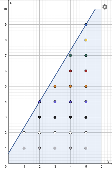
The sum above is equivalent to counting the number of lattice points below the curve $$$y = \frac{ax + b}{m}$$$ bounded by $$$0 \le x \lt n$$$. As an instance, the sum for $$$(a, b, m, n) = (3, 2, 5, 10)$$$ can be illustrated as follows.

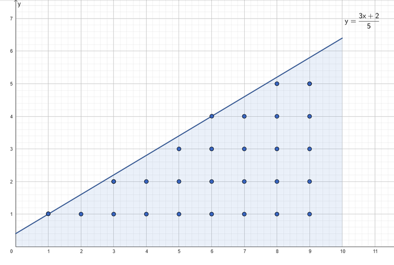
The goal here is to find another interpretation of the curve above, in the hope that we might find something useful. We can see that the lattice points are also to the "right" of the curve. If we try to rotate them:

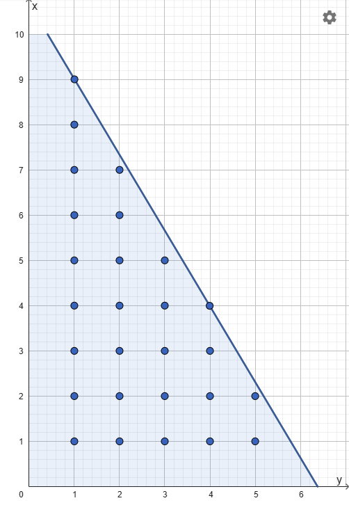
Now, we will try to relabel the rotated curve here so that it can fit to our definition of the function $$$S$$$.

Let $$$n' = \lfloor \frac{an + b}{m} \rfloor$$$. We notice that the curve covers $$$n'$$$ units of the $$$y$$$-axis. The curve at $$$y = n'$$$ is also $$$\frac{(an + b) \bmod m}{a}$$$ units away from the $$$y$$$-axis. Now, let's reflect the curve such it is pivoted at $$$y = n'$$$ instead.

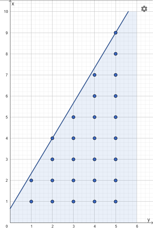
Now this looks like something we can represent with $$$S$$$. In fact, we can see that the curve now has slope $$$\frac{m}{a}$$$. If we let $$$b' = (an + b) \bmod m$$$, the number of lattice points below the curve above is exactly

To wrap, when $$$a \lt m$$$ and $$$b \lt m$$$, and letting $$$n' = \left\lfloor \frac{an + b}{m} \right\rfloor$$$ and $$$b' = (an + b) \bmod m$$$, we have:

This is good, because we just transformed $$$(a, m)$$$ into $$$(m, a)$$$, which in turn will be transformed into $$$(m \bmod a, a)$$$, then we can repeat the process. That is, $$$(a, m)$$$ will shrink like the Euclidean algorithm. We can stop when $$$S(a, b, m, n) = 0$$$, which will take $$$\mathcal O(\log m)$$$ steps.

2. Floor Sum Extension

In this section, we are going to compute the following:

and

Those two sums are going to be interrelated. We are going to, again, assume that $$$a \lt m$$$ and $$$b \lt m$$$. The case otherwise is left to the reader as an exercise.

Our goal here is the same as before: to swap $$$a$$$ and $$$m$$$ in its subproblem, so that $$$(a, m)$$$ will shrink like the Euclidean algorithm. For convenience, from this section onwards, we are also going to denote $$$n' = \lfloor \frac{an + b}{m} \rfloor$$$ and $$$b' = (an + b) \bmod m$$$.

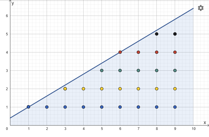
Let's start with visualising $$$T_1$$$:

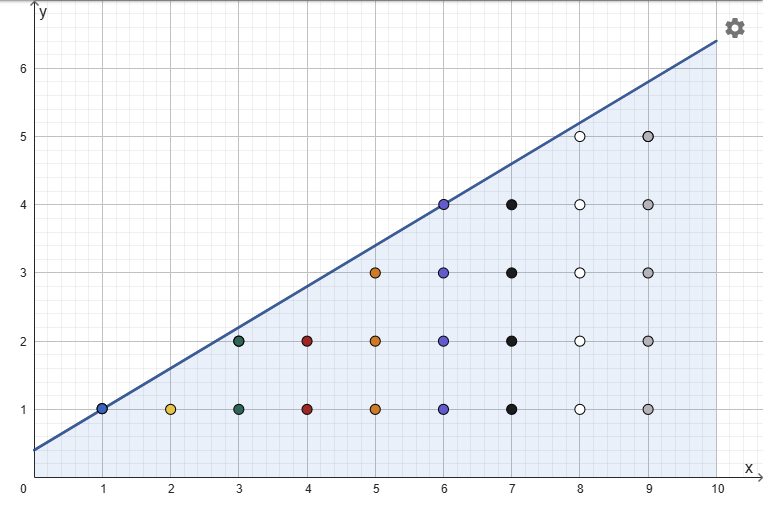
Here, the points have different colours for different contributions. In the illustration above, the colour-contributions are: (blue, $$$1$$$), (yellow, $$$2$$$), (green, $$$3$$$), and so on.

Let's transform the curve as we did in section 1.

Notice that, for each $$$y$$$, the contribution shrinks from bottom to top. The sum of point-by-point contributions based on the transformed curve is:

We have swapped $$$a$$$ and $$$m$$$ here, but now we have to compute $$$S_2$$$.

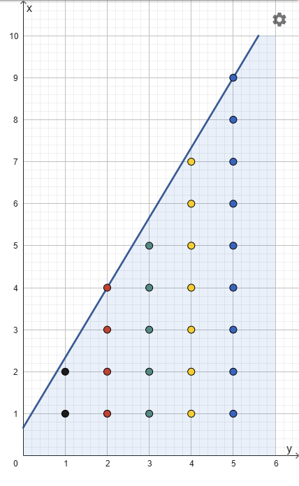
Let us now visualise $$$S_2$$$.

Here again, we are using different colours for different contributions. The contribution by the point at $$$(x, y)$$$ is $$$y^2 - (y-1)^2 = 2y - 1$$$. In this way, we can see that the sum of contributions for a fixed $$$x$$$ is exactly $$$\lfloor \frac{ax+b}{m}\rfloor^2$$$.

Transforming the curve above, we end up with

Let's sum the contributions based on this transformed curve.

and we are done.

Note that there will be overlapping subproblems, so it is a good idea to memoise the sums too. Since we will solve for $$$\mathcal O (\log m)$$$ subproblems of $$$S$$$, $$$T_1$$$, and $$$S_2$$$, the computation of both $$$T_1$$$ and $$$S_2$$$ can be done in $$$\mathcal O (\log m)$$$.

3. Bringing in the power

We are going to further extend the functions $$$T_1$$$ and $$$S_2$$$ by trying to compute:

and

The approach is exactly the same as the previous section, so you may refer to the same illustrations while reading this section, but the lattice points now have slightly more complex contributions as we are going to describe below.

It is also worth mentioning that $$$T_0 = S_1 = S$$$, so they can be evaluated like the floor sum from section 1 instead.

We start from $$$S_k$$$, since it is easier. The contribution by the point $$$(x, y)$$$ is $$$y^k - (y-1)^k$$$.

After the curve transformation,

so this single step takes $$$\mathcal O(k)$$$ to compute. Also note that we assume $$$0^0 = 1$$$ here.

For $$$T_k$$$, the contribution by the point $$$(x, y)$$$ is $$$x^k$$$. For this, we will define $$$P_d(n) = \sum_{x=0}^n x^d$$$. Using Faulhaber's formula,

where $$$B_i$$$ is the Bernoulli number whose generating function is $$$\frac{x}{e^x - 1}$$$.

The reason we are explicitly expanding the sum of powers will be more relevant at a later section. Back to computing $$$T_k$$$, after the curve transformation, we can then compute the contributions as follows.

The Bernoulli numbers can be precomputed, so this single step to compute $$$T_k$$$ also takes $$$\mathcal O(k)$$$ to compute.

Small Optimization

You may already notice that the formulas to compute $$$T_k$$$ and $$$S_k$$$ above involve convolutions. This means that, if we have already computed $$$T_i(m, b', a, n')$$$ and $$$S_i(m, b', a, n')$$$ (for all $$$0 \le i \le k$$$), then $$$T_i(a, b, m, n)$$$ and $$$S_i(a, b, m, n)$$$ (for all $$$0 \le i \le k$$$) can be computed in $$$\mathcal O(k \log k)$$$.

Back to computing $$$T_k$$$ and $$$S_k$$$, when you try to reduce for the case when $$$a \geq m$$$, you'll realise that you need to compute

which brings us to the next section.

4. Combining Everything Together

We are going to compute:

We just have to combine the expansions that we have obtained from the previous section. One can realise that the sum we want is:

which can be computed in $$$\mathcal O(k_1 k_2)$$$, so the overall operations to compute $$$S_{k_1, k_2}$$$ can be done in $$$\mathcal O ((k_1 + k_2)^4 \log m)$$$.

By noticing the convolution in the equation, and applying the optimisation we briefly mentioned from the previous section, it is, in fact, possible to bring down the whole operations to $$$\mathcal O((k_1 + k_2)^2 \log(k_1 + k_2) \log m)$$$.

Notes

From Min_25's article, it seems that it is possible to compute $$$S_k$$$ and $$$T_k$$$ in $$$\mathcal{O}(k^2 \log k)$$$ by decomposing $$$\frac{a}{m}$$$ using the Stern-Brocot tree. However, I am not sure whether there is an optimisation we can apply for our specific approach here without the need to compute $$$S_{k1, k2}$$$.

References

• Min_25's blog -- Scary Sum
• Floor Sum of Arithmetic Progression
• Wikipedia -- Faulhaber's Formula

Appendix

@functools.cache
def S(a, b, m, n):
    if a >= m:
        return (a // m) * n * (n - 1) // 2 + S(a % m, b, m, n)
    if b >= m:
        return (b // m) * n + S(a, b % m, m, n)

    n_, b_ = divmod(a*n + b, m)
    if n_ == 0:
        return 0

    return S(m, b_, a, n_)


@functools.cache
def T1(a, b, m, n):
    if a >= m:
        return (a // m) * (n - 1) * n * (2*n - 1) // 6 + T1(a % m, b, m, n)
    if b >= m:
        return (b // m) * n * (n - 1) // 2 + T1(a, b % m, m, n)

    n_, b_ = divmod(a*n + b, m)
    if n_ == 0:
        return 0

    return ((2 * n - 1) * S(m, b_, a, n_) - S2(m, b_, a, n_)) // 2


@functools.cache
def S2(a, b, m, n):
    if a >= m:
        return (a // m)**2 * (n - 1) * n * (2*n - 1) // 6 + 2 * (a // m) * T1(a % m, b, m, n) + S2(a % m, b, m, n)
    if b >= m:
        return (b // m)**2 * n + 2 * (b // m) * S(a, b % m, m, n) + S2(a, b % m, m, n) 

    n_, b_ = divmod(a*n + b, m)
    if n_ == 0:
        return 0

    return (2 * n_ - 1) * S(m, b_, a, n_) - 2 * T1(m, b_, a, n_)