


[cut]↵
** بسم الله والحمدلله والصلاة والسلام على رسول الله **↵
Bahnasy Tree↵
==================↵
**GitHub Repository:** [Bahnasy-Tree](https://github.com/Mostafa-Bahnasy/Bahnasy-Tree)↵
↵
Bahnasy Tree is a dynamic tree that represents a **sequence of length $N$** (positions $1..N$). It is controlled by two parameters:↵
↵
- $T$ ( **threshold** ): the maximum fanout a node is allowed to have before we consider it "too wide".↵
- $S$ ( **split factor** ): used when splitting; computed from the node size using the smallest prime factor (SPF). If $S > T$, we fallback to $S = 2$.↵
↵
The tree supports the usual sequence operations (find by index, insert, delete) and can be extended to support range query / range update by storing aggregates (sum, min, etc.) and optionally using lazy propagation.↵
↵
↵
---↵
↵
## 1) Node meaning and the main invariant↵
↵
Each node represents a contiguous block of the sequence. If a node represents a block of length `sz`, then its children partition this block into consecutive sub-blocks whose lengths sum to `sz`.↵
↵
The key invariant is: **every node always knows the sizes of its children subtrees** (how many leaves are inside each child).↵
↵
---↵
↵
## 2) Prefix sizes (routing by index)↵
↵
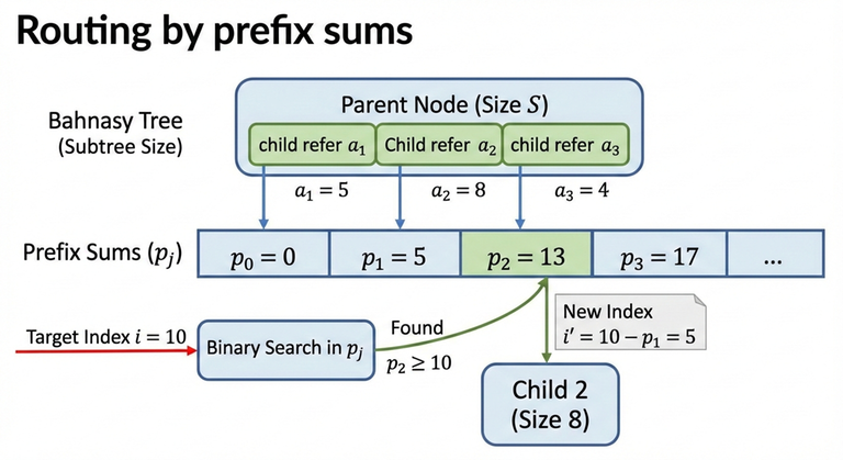
Assume a node has children with subtree sizes:↵
↵
$$a_1, a_2, \dots, a_k$$↵
↵
Define the prefix sums:↵
↵
$$p_0 = 0,\quad p_j = \sum_{t=1}^{j} a_t$$↵
↵
To route an index $i$ (1-indexed) inside this node:↵
↵
- Find the smallest $j$ such that $p_j \ge i$.↵
- Go to that child (and convert $i$ into the child-local index by subtracting $p_{j-1}$).↵
↵
Because $p_j$ is monotone, this is done using binary search ("lower bound on prefix sums").↵
↵
↵
---↵
↵
## 3) Building the tree (global split using SPF)↵
↵
Start with a root node representing $N$ elements.↵
↵
For a node representing $n$ elements:↵
↵
- If $n \le T$: stop splitting and create $n$ leaves under it.↵
- If $n > T$: split it into $S$ children:↵
- $S = \mathrm{SPF}(n)$↵
- If $S > T$, use $S = 2$↵
- Distribute the $n$ elements among those $S$ children (almost evenly), then recurse.↵
↵
This guarantees that during the initial build, every internal node has at most $T$ children.↵
↵
---↵
↵
## 4) Find / traverse complexity↵
↵
Define:↵
↵
- $D$: the depth (number of levels).↵
- At each level, routing uses binary search on at most $T$ children, so it costs $O(\log_2 T)$.↵
↵
Therefore:↵
↵
$$\mathrm{find} = O(D \cdot \log_2 T)$$↵
↵
In a "fully expanded" $T$-ary tree shape, depth is about:↵
↵
$$D \approx \log_T N$$↵
↵
So a direct expression is:↵
↵
$$\mathrm{find} = O(\log_T N \cdot \log_2 T)$$↵
↵
Now simplify using change-of-base:↵
↵
$$\log_T N = \frac{\log_2 N}{\log_2 T}$$↵
↵
Multiplying both sides by $\log_2 T$ gives:↵
↵
$$\log_T N \cdot \log_2 T = \log_2 N$$↵
↵
So the final form is:↵
↵
$$\mathrm{find} = O(\log_2 N)$$↵
↵
---↵
↵
## 5) Insert, local overflow, and local split↵
↵
Insertion happens at leaf level. After inserting a new element, the "leaf-parent" (the node whose children are leaves) increases its number of children.↵
↵
As long as the leaf-parent still has at most $T$ children, nothing structural is required.↵
↵
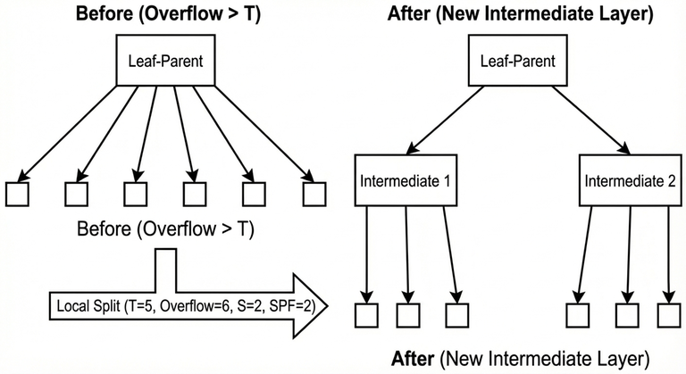
When the leaf-parent exceeds $T$ children, a **local split** is performed:↵
↵
- A new intermediate layer is created between the leaf-parent and its leaves.↵
- The old leaves are grouped into $S$ buckets (where $S$ is computed by the same SPF rule capped by $T$).↵
- This restores a bounded fanout and keeps future routing efficient.↵
↵
### Complexity of one local split↵
↵
A local split creates about $\mathrm{SPF}(T+1)$ intermediate nodes and reconnects about $T+1$ leaves, so ignoring the SPF term, the time is:↵
↵
$$O(T)$$↵
↵
### Insert complexity↵
↵
Insert cost is:↵
↵
- Routing: $O(\log_2 N)$↵
- Plus possible local overflow handling: $O(T)$↵
↵
So the worst-case insert is:↵
↵
$$O(\log_2 N + T)$$↵
↵
---↵
↵
## 6) Delete complexity↵
↵
Deletion also consists of:↵
↵
- Routing to the target: $O(\log_2 N)$↵
- Removing it from the leaf-parent's ordered child list (bounded by the same width idea), so $O(T)$↵
↵
So the worst-case delete is:↵
↵
$$O(\log_2 N + T)$$↵
↵
---↵
↵
## 7) Why rebuild is needed↵
↵
Repeated insertions concentrated in the same area can create a "deep path" because local splits keep adding intermediate layers.↵
↵
Consider the worst case where local splits behave like $S=2$:↵
↵
- After a local overflow, the leaves are grouped into 2 buckets of size about $T/2$.↵
- To overflow one bucket again and force another local split deeper, it takes about $T/2$ further insertions in that same region.↵
- Therefore, each new additional level costs about $T/2$ insertions.↵
↵
If the current depth is $D$ and the tree is considered valid only while $D \le T$, then the number of insertions needed to reach the invalid depth threshold is approximately:↵
↵
$$Y \approx (T - D)\cdot \frac{T}{2}$$↵
↵
In the worst case (starting from $D = 0$):↵
↵
$$Y \approx \frac{T^2}{2}$$↵
↵
When the tree becomes invalid, it is rebuilt.↵
↵
---↵
↵
## 8) Rebuild time↵
↵
A rebuild does:↵
↵
1. Collect leaves into an array of size $N$.↵
2. Reconstruct the tree from scratch using the global split rule.↵
↵
The rebuild time is proportional to the number of nodes created.↵
↵
Leaf level: $N$ nodes. ↵
Previous levels shrink geometrically, so the maximum total node count is bounded by:↵
↵
$$N + \frac{N}{2} + \frac{N}{4} + \frac{N}{8} + \dots$$↵
↵
Therefore rebuild cost is:↵
↵
$$O(N)$$↵
↵
---↵
↵
## 9) Total cost of rebuilds across $Q$ operations↵
↵
In the worst case, rebuild happens every $\Theta(T^2)$ insertions concentrated in one place.↵
↵
So number of rebuilds is approximately:↵
↵
$$\frac{Q}{T^2}$$↵
↵
Each rebuild costs $O(N)$, therefore total rebuild time across all operations is:↵
↵
$$O\!\left(\frac{NQ}{T^2}\right)$$↵
↵
For operation costs in the same worst-style view, insertion can be treated as $O(T)$ due to local split work, so the operation part is:↵
↵
$$O(QT)$$↵
↵
Thus a total bound is:↵
↵
$$O\!\left(\frac{NQ}{T^2} + QT\right)$$↵
↵
---↵
↵
## 10) Choosing a good $T$↵
↵
A common practical choice is:↵
↵
$$T \approx \sqrt[3]{N}$$↵
↵
Because plugging $T = N^{1/3}$ into the rebuild term:↵
↵
$$\frac{NQ}{T^2} = \frac{NQ}{N^{2/3}} = QN^{1/3}$$↵
↵
and the operations term $QT$ becomes:↵
↵
$$QT = QN^{1/3}$$↵
↵
so both terms become the same order:↵
↵
$$O(Q\sqrt[3]{N})$$↵
↵
In practice (based on testing), good values often fall in the range:↵
↵
$$T \in [N^{0.27},\, N^{0.39}]$$↵
↵
with higher values helping insertion-heavy workloads and lower values helping query-heavy workloads.↵
↵
---↵
↵
## 11) Worst-case tests and mitigation↵
↵
Worst-case behavior happens when a test is engineered to keep inserting in exactly the same place so the tree reaches a depth close to $T$, and then many operations are issued around that hot region.↵
↵
Common mitigations:↵
↵
- Randomize $T$ each rebuild within a safe exponent range (e.g. $N^{0.27}$ to $N^{0.39}$).↵
- Randomize the rebuild target (instead of rebuilding exactly at depth $T$, rebuild at $(0.5/1/2/3/4)\cdot T$).↵
↵
---↵
↵
## 12) Implementations↵
↵
**Minimal structure-only implementation** (split / split_local / find / insert / delete): ↵
[general_structure.cpp](https://github.com/Mostafa-Bahnasy/Bahnasy-Tree/blob/main/src/Bahnasy%20Tree%20src/Generic/general_structure.cpp)↵
↵
**Full implementation** (find/query/update/insert/delete + rebuild): ↵
[non_generic_version.cpp](https://github.com/Mostafa-Bahnasy/Bahnasy-Tree/blob/main/src/Bahnasy%20Tree%20src/competitive%20programming/non_generic_version.cpp)↵
↵
---↵
↵
## Benchmark results↵
↵
Stress-testing results comparing Bahnasy Tree implementations against Treap and Segment Tree showed **full agreement** (no diffs) across all test suites.↵
↵
| Test suite | Bahnasy variant | Reference | Tests | Bahnasy avg time | Reference avg time |↵
|---|---|---|---:|---|---|↵
| All operations | non_generic_version.cpp | treap_fast.cpp | 105 | 0.202s | 0.193s |↵
| Point update + query | bahnasy_point_update.cpp | segTree_point_update.cpp | 18 | 0.303s | 0.218s |↵
| Range update + query | bahnasy_range_update.cpp | segTree_range_update.cpp | 12 | 0.274s | 0.236s |↵
↵
Full benchmark logs and automated testing scripts are available in the GitHub repository under `tools/` and `reports/`.↵
↵
**Tutorials:** ↵
↵
[Bahnasy-Tree-Arabic-Readers](https://www.youtube.com/watch?v=ENVNiOvHJrA)↵
↵
[Bahnasy-Tree-English-Readers](https://youtu.be/n3FDxEaFS_0)↵
↵
[Paper](https://doi.org/10.13140/RG.2.2.13888.60165)↵
↵
** بسم الله والحمدلله والصلاة والسلام على رسول الله **↵
Bahnasy Tree↵
==================↵
**GitHub Repository:** [Bahnasy-Tree](https://github.com/Mostafa-Bahnasy/Bahnasy-Tree)↵
↵
Bahnasy Tree is a dynamic tree that represents a **sequence of length $N$** (positions $1..N$). It is controlled by two parameters:↵
↵
- $T$ ( **threshold** ): the maximum fanout a node is allowed to have before we consider it "too wide".↵
- $S$ ( **split factor** ): used when splitting; computed from the node size using the smallest prime factor (SPF). If $S > T$, we fallback to $S = 2$.↵
↵
The tree supports the usual sequence operations (find by index, insert, delete) and can be extended to support range query / range update by storing aggregates (sum, min, etc.) and optionally using lazy propagation.↵
↵
↵
---↵
↵
## 1) Node meaning and the main invariant↵
↵
Each node represents a contiguous block of the sequence. If a node represents a block of length `sz`, then its children partition this block into consecutive sub-blocks whose lengths sum to `sz`.↵
↵
The key invariant is: **every node always knows the sizes of its children subtrees** (how many leaves are inside each child).↵
↵
---↵
↵
## 2) Prefix sizes (routing by index)↵
↵
Assume a node has children with subtree sizes:↵
↵
$$a_1, a_2, \dots, a_k$$↵
↵
Define the prefix sums:↵
↵
$$p_0 = 0,\quad p_j = \sum_{t=1}^{j} a_t$$↵
↵
To route an index $i$ (1-indexed) inside this node:↵
↵
- Find the smallest $j$ such that $p_j \ge i$.↵
- Go to that child (and convert $i$ into the child-local index by subtracting $p_{j-1}$).↵
↵
Because $p_j$ is monotone, this is done using binary search ("lower bound on prefix sums").↵
↵
↵
---↵
↵
## 3) Building the tree (global split using SPF)↵
↵
Start with a root node representing $N$ elements.↵
↵
For a node representing $n$ elements:↵
↵
- If $n \le T$: stop splitting and create $n$ leaves under it.↵
- If $n > T$: split it into $S$ children:↵
- $S = \mathrm{SPF}(n)$↵
- If $S > T$, use $S = 2$↵
- Distribute the $n$ elements among those $S$ children (almost evenly), then recurse.↵
↵
This guarantees that during the initial build, every internal node has at most $T$ children.↵
↵
---↵
↵
## 4) Find / traverse complexity↵
↵
Define:↵
↵
- $D$: the depth (number of levels).↵
- At each level, routing uses binary search on at most $T$ children, so it costs $O(\log_2 T)$.↵
↵
Therefore:↵
↵
$$\mathrm{find} = O(D \cdot \log_2 T)$$↵
↵
In a "fully expanded" $T$-ary tree shape, depth is about:↵
↵
$$D \approx \log_T N$$↵
↵
So a direct expression is:↵
↵
$$\mathrm{find} = O(\log_T N \cdot \log_2 T)$$↵
↵
Now simplify using change-of-base:↵
↵
$$\log_T N = \frac{\log_2 N}{\log_2 T}$$↵
↵
Multiplying both sides by $\log_2 T$ gives:↵
↵
$$\log_T N \cdot \log_2 T = \log_2 N$$↵
↵
So the final form is:↵
↵
$$\mathrm{find} = O(\log_2 N)$$↵
↵
---↵
↵
## 5) Insert, local overflow, and local split↵
↵
Insertion happens at leaf level. After inserting a new element, the "leaf-parent" (the node whose children are leaves) increases its number of children.↵
↵
As long as the leaf-parent still has at most $T$ children, nothing structural is required.↵
↵
When the leaf-parent exceeds $T$ children, a **local split** is performed:↵
↵
- A new intermediate layer is created between the leaf-parent and its leaves.↵
- The old leaves are grouped into $S$ buckets (where $S$ is computed by the same SPF rule capped by $T$).↵
- This restores a bounded fanout and keeps future routing efficient.↵
↵
### Complexity of one local split↵
↵
A local split creates about $\mathrm{SPF}(T+1)$ intermediate nodes and reconnects about $T+1$ leaves, so ignoring the SPF term, the time is:↵
↵
$$O(T)$$↵
↵
### Insert complexity↵
↵
Insert cost is:↵
↵
- Routing: $O(\log_2 N)$↵
- Plus possible local overflow handling: $O(T)$↵
↵
So the worst-case insert is:↵
↵
$$O(\log_2 N + T)$$↵
↵
---↵
↵
## 6) Delete complexity↵
↵
Deletion also consists of:↵
↵
- Routing to the target: $O(\log_2 N)$↵
- Removing it from the leaf-parent's ordered child list (bounded by the same width idea), so $O(T)$↵
↵
So the worst-case delete is:↵
↵
$$O(\log_2 N + T)$$↵
↵
---↵
↵
## 7) Why rebuild is needed↵
↵
Repeated insertions concentrated in the same area can create a "deep path" because local splits keep adding intermediate layers.↵
↵
Consider the worst case where local splits behave like $S=2$:↵
↵
- After a local overflow, the leaves are grouped into 2 buckets of size about $T/2$.↵
- To overflow one bucket again and force another local split deeper, it takes about $T/2$ further insertions in that same region.↵
- Therefore, each new additional level costs about $T/2$ insertions.↵
↵
If the current depth is $D$ and the tree is considered valid only while $D \le T$, then the number of insertions needed to reach the invalid depth threshold is approximately:↵
↵
$$Y \approx (T - D)\cdot \frac{T}{2}$$↵
↵
In the worst case (starting from $D = 0$):↵
↵
$$Y \approx \frac{T^2}{2}$$↵
↵
When the tree becomes invalid, it is rebuilt.↵
↵
---↵
↵
## 8) Rebuild time↵
↵
A rebuild does:↵
↵
1. Collect leaves into an array of size $N$.↵
2. Reconstruct the tree from scratch using the global split rule.↵
↵
The rebuild time is proportional to the number of nodes created.↵
↵
Leaf level: $N$ nodes. ↵
Previous levels shrink geometrically, so the maximum total node count is bounded by:↵
↵
$$N + \frac{N}{2} + \frac{N}{4} + \frac{N}{8} + \dots$$↵
↵
Therefore rebuild cost is:↵
↵
$$O(N)$$↵
↵
---↵
↵
## 9) Total cost of rebuilds across $Q$ operations↵
↵
In the worst case, rebuild happens every $\Theta(T^2)$ insertions concentrated in one place.↵
↵
So number of rebuilds is approximately:↵
↵
$$\frac{Q}{T^2}$$↵
↵
Each rebuild costs $O(N)$, therefore total rebuild time across all operations is:↵
↵
$$O\!\left(\frac{NQ}{T^2}\right)$$↵
↵
For operation costs in the same worst-style view, insertion can be treated as $O(T)$ due to local split work, so the operation part is:↵
↵
$$O(QT)$$↵
↵
Thus a total bound is:↵
↵
$$O\!\left(\frac{NQ}{T^2} + QT\right)$$↵
↵
---↵
↵
## 10) Choosing a good $T$↵
↵
A common practical choice is:↵
↵
$$T \approx \sqrt[3]{N}$$↵
↵
Because plugging $T = N^{1/3}$ into the rebuild term:↵
↵
$$\frac{NQ}{T^2} = \frac{NQ}{N^{2/3}} = QN^{1/3}$$↵
↵
and the operations term $QT$ becomes:↵
↵
$$QT = QN^{1/3}$$↵
↵
so both terms become the same order:↵
↵
$$O(Q\sqrt[3]{N})$$↵
↵
In practice (based on testing), good values often fall in the range:↵
↵
$$T \in [N^{0.27},\, N^{0.39}]$$↵
↵
with higher values helping insertion-heavy workloads and lower values helping query-heavy workloads.↵
↵
---↵
↵
## 11) Worst-case tests and mitigation↵
↵
Worst-case behavior happens when a test is engineered to keep inserting in exactly the same place so the tree reaches a depth close to $T$, and then many operations are issued around that hot region.↵
↵
Common mitigations:↵
↵
- Randomize $T$ each rebuild within a safe exponent range (e.g. $N^{0.27}$ to $N^{0.39}$).↵
- Randomize the rebuild target (instead of rebuilding exactly at depth $T$, rebuild at $(0.5/1/2/3/4)\cdot T$).↵
↵
---↵
↵
## 12) Implementations↵
↵
**Minimal structure-only implementation** (split / split_local / find / insert / delete): ↵
[general_structure.cpp](https://github.com/Mostafa-Bahnasy/Bahnasy-Tree/blob/main/src/Bahnasy%20Tree%20src/Generic/general_structure.cpp)↵
↵
**Full implementation** (find/query/update/insert/delete + rebuild): ↵
[non_generic_version.cpp](https://github.com/Mostafa-Bahnasy/Bahnasy-Tree/blob/main/src/Bahnasy%20Tree%20src/competitive%20programming/non_generic_version.cpp)↵
↵
---↵
↵
## Benchmark results↵
↵
Stress-testing results comparing Bahnasy Tree implementations against Treap and Segment Tree showed **full agreement** (no diffs) across all test suites.↵
↵
| Test suite | Bahnasy variant | Reference | Tests | Bahnasy avg time | Reference avg time |↵
|---|---|---|---:|---|---|↵
| All operations | non_generic_version.cpp | treap_fast.cpp | 105 | 0.202s | 0.193s |↵
| Point update + query | bahnasy_point_update.cpp | segTree_point_update.cpp | 18 | 0.303s | 0.218s |↵
| Range update + query | bahnasy_range_update.cpp | segTree_range_update.cpp | 12 | 0.274s | 0.236s |↵
↵
Full benchmark logs and automated testing scripts are available in the GitHub repository under `tools/` and `reports/`.↵
↵
**Tutorials:** ↵
↵
[Bahnasy-Tree-Arabic-Readers](https://www.youtube.com/watch?v=ENVNiOvHJrA)↵
↵
[Bahnasy-Tree-English-Readers](https://youtu.be/n3FDxEaFS_0)↵
↵
[Paper](https://doi.org/10.13140/RG.2.2.13888.60165)↵
↵

