Stop doing MHC R3 that's not what matters!
№ | Пользователь | Рейтинг |
---|---|---|
1 | tourist | 4009 |
2 | jiangly | 3823 |
3 | Benq | 3738 |
4 | Radewoosh | 3633 |
5 | jqdai0815 | 3620 |
6 | orzdevinwang | 3529 |
7 | ecnerwala | 3446 |
8 | Um_nik | 3396 |
9 | ksun48 | 3390 |
10 | gamegame | 3386 |
Страны | Города | Организации | Всё → |
№ | Пользователь | Вклад |
---|---|---|
1 | cry | 167 |
2 | Um_nik | 163 |
3 | maomao90 | 162 |
3 | atcoder_official | 162 |
5 | adamant | 159 |
6 | -is-this-fft- | 158 |
7 | awoo | 157 |
8 | TheScrasse | 154 |
9 | Dominater069 | 153 |
9 | nor | 153 |
Stop doing MHC R3 that's not what matters!
An OpenAI model can now achieve a rating of 1800 in Codeforces. That made me wonder about the future of competitive programming and why we do this. I came up with some opinions, which I'll be glad to share with you.
I don't think that's happening, because competitive programming is useless! Some people might think CP is less interesting because AI can solve CP problems — but come on, problemsetter can solve those problems, unless they are really bad. Many people still play Chess just fine, and I recently enjoyed participating in Sudoku competitions, although I was completely aware that computers would wreck me in a second. It didn't matter, and I didn't see how it could.
CP problems are not "open problems" — if they are, the problemsetters are to blame. So, you are not contributing anything to the world by solving CP problems; it all comes down to personal interest. As long as CP is fun for people, they will do it.
They are onsite competition — they can stop people from using AI to solve problems, and according to their records (IOI banning all prewritten codes, ICPC only allowing teamnotes), they will. They will stay as is.
I want to note that the situation is already quite dire for those contests. GCJ is gone, MHC is still not recovering from virtual, Topcoder is gone, and AtCoder is less frequent; it's no secret we are going downhill.
I also think the contest integrity is already under attack, especially in the last five post-COVID years. No need to mention thousands of low-rated cheaters in CF. High-rated people also cheat (1 2).
Given all the records, a nonnegligible amount of people, regardless of their skill level, will try to cheat in various online contests with AI. That is not good news for CF and AtCoder, which partially or fully bans the use of AI.
Another argument is that it is still fair game if everyone uses it. For example, Internet search is allowed in CF, and notably, I took advantage of that. To whatever extent how it trivializes CP, everyone can use AI nowadays; what's the issue?
I think allowing AI is a fair game, but I wonder if it's a good game. Some issues I have with it:
One way to delay these impacts is to propose problems that AI can not solve by now. I think this is a bad trade.
A problem should be judged independently over how well AI can solve it, and it's the right call to ban AI in online contests. Then, a CF rating will "really" be a number, similar to the online judge rankings. You can say it already is, but I bet I never saw a single high-rated user who literally considered it as just numbers without an ego attached, so get ready for some changes.
If I'm being sincere, probably not.
One clear example is interviews. However, most corporate interviews don't ask about CP problems because they do CP at work. They will figure out some way if AI cheat is prevalent, so not our business.
Ok, those are boring talk. Why do people like competitive programming? I would imagine the following:
The AI revolution will harm the third point as they will win less, but that's ok. That's not a healthy mindset, anyway.
For the other points, it even seems that competitive programming where we have AI assistance is a better idea, as long as you are using it for practice only — you can ask and learn cool new things from AI, as it will gather thousands of information and pick you the right one.
Problem-wise, no, I think that's a bad idea, as I wrote earlier.
But we will see some changes. I predict that AI will contribute to the slow demise of online contests by harming their integrity even further — Many people, including me, will miss Codeforces, where the rating isn't a completely random number, and admire tourist for having such a high rating, so this is indeed a bad thing.
I also think the idea of "infinite resources" makes less sense. Before AI, I thought a contest allowing all possible human resources was an ideal model, and we should judge our skills based on that. Now, I feel that there should be a limitation to this, as what IOI and ICPC have been doing. I'm not entirely sure about this.
On the bright side, you should think of the rating as just a number, so this change might be a good thing, as it makes us keep the right mindset for competition.
Final Results are out! Congratulations to everyone, especially:
IOI 2024 is held in Alexandria, Egypt. Good luck to all participants! I'm also attending as a student coach (Guest) as well; please say hi if you see me!
All times are in UTC+3 (Egypt — Eastern European Summer Time).
Links
Please, keep all discussions civil and according to the IOI Code of Conduct. Please.
bobr_babizon posted an article, a machine translation of a Kinetic Segment Tree post in my Korean blog. Given this interest in my small Korean blog, I felt obliged to introduce it.
In most of my undergrad period, I was sponsored by the generous Samsung Software Membership, where one of their remarkable features was to fund "individual research projects" — In short, each month, I write an article on interesting stuff, and they will pay me 500,000 KRW per article. Amazing, as it motivates me to learn new stuff and also get paid.
Here is the full list of posts written by that initiative.
Not all posts are good. Sometimes, I need to keep up with the deadline and rush the post; sometimes, I write stuff in specific interest; sometimes, the topic is too hard and I only obtain a superficial understanding. But there are some posts, which I think are the best posts on their subject matter for CF audience if translated into English:
Sometimes I actually posted them in English:
Why are all these posts in Korean? It's because the sponsor wanted such a way — otherwise, I'd actually write all of them in English. So that's pretty sad, and I don't think I will ever try to translate them, but I hope someone would still find them helpful.
The World Finals are right ahead, and if everything works as I expect, you will probably have to wait a lot of time before the contest, dress rehearsals, or anything else. I prepared this blog post so that you have something to keep yourself occupied.
Our goal is to maintain connectivity in fully-dynamic query streams. In other words, we want to solve this problem:
The offline version, where you can cheat (aka, read all queries before answering, and answer everything at the very end of the program) has a very cool solution commonly known as Offline Dynamic Connectivity. This is enough in most CP problems, where this offline solution is rarely considered cheating.
Unfortunately, people in the academia are not chilling and consider this a kind of cheating (not exactly but w/e), so we need to respond to each query right after they are given. This is known as Online Dynamic Connectivity or HDLT Algorithm. I think it is as well-known as the offline algorithm in the sense that people know it exists, but many people just think it's way too hard.
The dynamic connectivity problem can be solved if the underlying graph is guaranteed to be a forest. Indeed, in this case, you can do a little bit more than just maintaining the connectivity, you can (and you have to) do the following:
link(u, v)
: Insert an edge $$$e = (u, v)$$$ into a forest, given that the graph remains a forest.cut(u, v)
: Delete an edge $$$e = (u, v)$$$ from a forest.find_root(u)
: Returns a root node of a component of $$$u$$$ — it is basically some random node that is consistently returned among the component (just like the find
operation in DSU)sum(u)
: Returns a sum of labels in a component of $$$u$$$ (yes, each vertex is associated with some labels)find_first(u)
: Returns the first node in a component of $$$u$$$ that satisfies some predicate (per labels).update(v, x)
: Update the label of $$$v$$$ to $$$x$$$This is pretty easy if you have a good top tree implementation by ecnerwala and know how to use it. But if you don't, then you have to use a sad BBST that maintains this weird cyclic Euler tree order and oh so confusing. But I'm not writing a top tree tutorial here, so let's not delve into these technicalities.
We do want to leverage the fact that a spanning forest can be maintained — so let's try to maintain a spanning forest and the set of back edges that currently do not belong to that spanning forest (but can be later if some edges are deleted)
Insertion is as easy as DSU — check if find_root(u) != find_root(v)
. If it is, add into a spanning forest with link
operation. Otherwise throw it into the list of back edges. Easy!
Or is it? Suppose the deleted edge are one of the back edges. Then you can just remove them from the set and call it a day.
Suppose not. Then use the cut
operation to remove the edge from the forest. After the removal of the edge, the component will be split into two parts. Some back edge may connect these two parts, and in that case, you have to insert them into the spanning forest again.
So you have to find a back edge that connects these two parts. This looks easy, can't you just use some segment trees in Euler tours? Well, the fact that trees are dynamic makes it very hard to solve this problem, especially given that nobody has any idea on how to tackle the problem this way.
And now we found the devil. We have to find the back edges between these two parts quickly.
Given that it seems hard to directly find the edge between two component, another approach to solve this is by scanning each edge at most once — then, although in each query you may spend a lot of time, the total time spent will be at most the number of (inserted) edges, which looks good.
Let's try this. For each vertex, label them with the number of back edges incident with it. After removing the edge $$$(u, v)$$$, let $$$T_u, T_v$$$ be the component connecting each vertices. We scan each $$$T_u$$$'s back edges (using find_first
) . If they connect $$$T_u$$$ and $$$T_v$$$, we are done!
Otherwise, we need to not scan them again, what should we do? Well, just throw them away! And get wrong answer. But we want to throw them away so badly, how should we do?
The kicker here is that we can assume $$$|T_u| \le |T_v|$$$ here. Anyway, the choice of $$$T_u$$$ was pretty random, and we can know the size of the subtree by storing as one of labels in top tree. And that means $$$|T_u| \le \frac{1}{2} (|T_u| + |T_v|)$$$, so we want to kick out those edges into this small area and somehow hope that we won't be kicking out each edges too much. Like, if this area is "really small" like $$$|T_u| = 1$$$, the back edge won't even exist. So we hope to scan each edge at most $$$\log n$$$ time, hopefully.
Here's our strategy. We want to push down each back edges if they ended up not connecting the tree again. Let's do it for only two layers. Suppose that we have some back edges that we don't want to scan. What should we do? If we only push down back edges, it's just a heap of random edges. So we also need to push down the tree as well. Let's push all tree edges of $$$T_u$$$ as well.
Then we have an algorithm. Let's say the upper layer is the main layer we are working, and the lower layer is the smaller layer where we throw stuff away. Here are the two invariants we are maintaining:
In the insertion case, just add the edge in the upper layer. Easy.
In the deletion case, let's analyze the cases:
So far so good, If nothing in lower layer fails, we already has an algorithm.
Let's generalize the above algorithm so that we can repeat the same argument even if the edge in the lower layer fails. We have
As an invariant, each edge set of forest in layer $$$i+1$$$ is a subset of that in layer $$$i$$$.
Insertion is still easy; add an edge in layer $$$0$$$.
In the deletion case, let's analyze the cases:
Now, every time we touch the edge, we increase their level. This level can't go over $$$\log n$$$, and top tree has $$$O(\log n)$$$ time, so we obtain a $$$O(\log^2 n)$$$ amortized time algorithm. Not easy, but very simple!
Hello Codeforces! I just uploaded the first paper of my life to arXiv, and I'm happy to share this with the community, especially because it is very related to competitive programming.
Here is the presentation I gave in MIT Theory Lunch.
Everyone knows the Floyd-Warshall algorithm for computing the shortest path, it goes like this:
rep(k, n) rep(i, n) rep(j, n) A[i][j] = min(A[i][j], A[i][k] + A[k][j]);
And everyone knows this incorrect variant of Floyd-Warshall. I certainly implemented this when I was learning CP, cause I kinda wanted to "fix the loop order".
rep(i, n) rep(j, n) rep(k, n) A[i][j] = min(A[i][j], A[i][k] + A[k][j]);
This is bad, it does not compute the shortest path. It does, however, compute "something". Imagine someone gives you a sparse graph and asks you to compute "something". Then that's actually harder than the correct variant because you can't run Dijkstra! What is this?!
But don't worry, with some observation, you can actually run some sort of Dijkstra:
Theorem 1.2: The "incorrect Floyd-Warshall matrix" can be computed with a single Dijkstra and a simple DP.
Then there's this really funny preprint by DEGwer and EnumerativeCombinatorics which basically says that "nobody cares about loop order cause you can run incorrect ones $$$3$$$ times." This makes total sense when you want to compute the correct matrix in a troll way. But what about the other way around? What if you want to compute the troll matrix, given that you can only use a very serious black box of Floyd-Warshall?
Theorem 1.3: The "incorrect Floyd-Warshall matrix" can be computed with $$$O(\log n)$$$ iteration of Floyd-Warshall plus $$$O(n^2 \log n)$$$ computation.
This is quite interesting if you have a context — it is conjectured that the all-pair shortest path can't be computed faster than $$$O(n^3)$$$ (by Floyd-Warshall) and breaking it will be a major breakthrough. Like NP-Complete, there are a group of problems classified as "APSP-Complete" if a subcubic solution in one of them implies subcubic solution for everything. I just added a little troll problem in that list.
In late January, I was in NYC and was sleeping on ksun48's couch. In the afternoon we wanted to have some fun, so I created a random Baekjoon OJ mashup, and one of those random problems was from the PA 2019 finals. We both spent quite a lot of time on this problem but could not solve it before I had to leave for dinner, which was weird because it didn't seem impossible per PtzCamp standings. Anyway, I upsolved it later (which later became proof of my Thm 1.2), and then I realized the intended solution is a bitset cheese, lol
The MIT theory group has this "30-minute lunch talk" where there is free food, and people discuss random stuff. In February there were not a lot of people giving a talk, and it was the beginning of semester so I think some troll CP stuff can be tolerated. So I prepared that presentation and gave a talk (at this point I had almost zero intention on publishing this on conference).
After the talk, jcvb informed me of a conference called "Fun with Algorithms" where I can actually publish these. Technically, as the intended one was bitset cheese, I have an original solution (amplified by the fact that ksun48 did not gave me hint even though I asked, wtf), so if I can overcome the tight deadline it was kind of a good idea. But that time, I only had Theorem 1.2, and submitting it looked a little disrespectful to this DEGwer paper, so I tried to prove Theorem 1.3. I succeeded, and it looked pretty good to me, so I submitted it and got an acceptance.
This question striked my head: "How can I solve dynamic $$$k$$$-connectivity efficiently?"
And then I tried to answer it, but I realized that my question was open to a lot of different interpretations.
Two vertices are $$$k$$$-connected if there are $$$k$$$ edge-disjoint paths connecting two vertices. For $$$k = 1$$$, it is the usual definition of connectivity.
If I say, "I solved the graph connectivity problem", what can it possibly mean?
First Interpretation ($$$s$$$-$$$t$$$ connectivity). I can respond to the following query efficiently: Given two vertices $$$s, t$$$, determine if there is a path between them. In the case of $$$k = 1$$$, graph search suffices.
What about higher $$$k$$$? You can find $$$k$$$ edge-disjoint path by reducing it into a flow problem. Each edge-disjoint path corresponds to a flow from $$$s$$$-$$$t$$$, so make all edges to capacity one, and find a flow of total capacity $$$k$$$ from $$$s$$$ to $$$t$$$. This algorithm takes $$$O(\min(k, m^{1/2}) (n + m))$$$ time.
Second Interpretation (Graph connectivity). I can't respond to an individual query, but I can respond if all pairs of vertices are connected or not. In the case of $$$k = 1$$$, the answer is true if the graph is connected. In the case of $$$k = 2$$$, the answer is true if the graph is connected and has no bridges.
In higher $$$k$$$, the problem is problem is known as Global Min Cut. How to solve it?
Third Interpretation (Connectivity Certificate). It sucks to have only one of them, why not both? In the case $$$k = 1$$$, we can DFS for each connected component and label it, so $$$s$$$-$$$t$$$ connectivity is solved by checking if $$$label[u] = label[v]$$$, and graph connectivity is solved by checking if all labels are same. In the case $$$k = 2$$$, we can compute the biconnected component of the graph (aka remove bridges and DFS) to do the same thing. So we have this theme:
Another important structure is the Gomory-Hu Tree. For an undirected graph, there is a tree with the same vertex set and weighted edges, where the $$$s-t$$$ max flow corresponds to the minimum weight in the unique $$$s-t$$$ path in the tree. This also works as a good certificate, since the $$$s - t$$$ path minimum can be computed efficiently with sparse tables or likewise. A standard way to compute the Gomory-Hu tree requires $$$n$$$ iteration of the maximum flow algorithm, which is $$$O(m^{3/2})$$$ assuming a standard algorithm in an unweighted case.
How to maintain such certificate in dynamic queries? Suppose that you have two big connected components, and you repeatedly add and remove edges between those components. If you maintain a dynamic graph under such a label, then you will end up with $$$O(n)$$$ labels changing in each query which is clearly impossible. I assume the certificate as an implicit structure (Disjoint Set Union, Link Cut Tree are good examples) that preserves the connectivity structure without a few changes and can answer some queries (component aggregates, root/label of the component) in an efficient ways. This is kinda ill-defined, but I don't know how to formalize it.
Still more interpretation? You can define connectivity as the minimum number of vertex to remove. For such a definition, there are a lot of interesting structures such as Block-Cut Tree or SPQR Tree, but the margin is too short to contain these. I limit the scope of the article to exact undirected edge connectivity, which is still not enough to make this article exhaustive, but whatever.
Mostly, if we say a graph is dynamic, then we assume updates that insert and delete the edges. This is known as fully-dynamic, but this may get too hard and sometimes we may resort to special cases such as incremental and decremental. The case of incremental assumes no update that deletes the edges, and for the decremental — no updates that insert the edges. For example, disjoint set union (DSU) solves the connectivity problem in case the updates are incremental.
Sometimes, you don't have to answer all queries immediately, but only before the program terminates. In that case, you can take advantage of the fact that you know the whole set of queries that will be given, and may change the order of computations or so on. This setting is called offline and it is especially prevalent in competitive programming. For example, the connectivity problem can be solved fully-dynamic if we assume offline queries, and this idea is well-known under the name Offline Dynamic Connectivity.
Another interesting special case is where the updates are not cumulative: Given a graph, you add or remove a small set of vertex/edges, respond to the query, and then the update queries are reverted and you get back to the original graph given. For example, you may want to know if there is a $$$s - t$$$ path if edge $$$e$$$ is removed from the graph — you can solve this with biconnected components. This setting is called sensitivity, which is not prevalent in CP, but I know problems that ask this (problem G).
And of course, there is freedom over the selection of $$$k$$$ as well. $$$k$$$ could be either $$$1$$$ (connectivity), $$$2$$$ (biconnectivity), $$$3$$$ (triconnectivity), $$$4$$$ (??), $$$O(1), O(\text{poly}(\log n))$$$, $$$O(n)$$$ .. it could be even very bigger if you assume that edges are weighted and define connectivity as the maximum $$$s - t$$$ flow.
But there should be no dispute about the efficiency since it's just fast or slow. Is it? Maybe not. Sometimes, you are concerned about the worst-case query time, where you have to answer all queries with small computation. At other times, you are concerned about the amortized query time, where each query may need long computation, but in the end, the sum of spent computation can be bounded.
Worst-case bound can be necessary not only by itself but also when you need to use it as a black-box data structure. Suppose you want to support the undoing of the last query, or even make it persistent. Then you can take some queries that need long computation, undo and redo repeatedly to mess up the analysis.
The efficiency can have different definitions in diverse computing environments such as parallel / distributed, which we won't go into for obvious reasons.
So we have these various measures, let's make some tables! Please write in comments if the results are incorrect or not the fastest. The table is just a collection of googled materials.
All results below assume amortized bounds. I omitted Big-O for brevity.
$$$k$$$ | $$$s - t$$$ | Global | Certificate |
---|---|---|---|
$$$1$$$ | $$$m$$$ [1] | $$$m$$$ [1] | $$$m$$$ [1] |
$$$2$$$ | $$$m$$$ [2] | $$$m$$$ [5] | $$$m$$$ [5] |
$$$3$$$ | $$$m$$$ [2] | $$$m$$$ [6] | $$$m$$$ [6] |
$$$4$$$ | $$$m$$$ [2] | $$$m$$$ [7] | $$$m$$$ [7] |
$$$O(1)$$$ | $$$m$$$ [2] | $$$m + n \log n$$$ [9] | $$$m + n \log n$$$ [9] |
$$$\text{poly} \log n$$$ | $$$m \text{ poly}\log n$$$ [2] | $$$m \log^2 n$$$ [4] | $$$(m + n) \text{ poly} \log n$$$ [9] |
$$$O(n)$$$ | $$$m^{1 + o(1)}$$$ [3] | $$$m \log^2 n$$$ [4] | $$$m^{1 + o(1)}$$$ [8] |
Weighted | $$$m^{1 + o(1)}$$$ [3] | $$$m \log^2 n$$$ [4] | $$$n^2 \text{ poly} \log n$$$ [8] |
$$$k$$$ | $$$s - t$$$ | Global | Certificate |
---|---|---|---|
$$$1$$$ | $$$\log n$$$ [10] | $$$\log n$$$ [10] | $$$\log n$$$ [10] |
$$$2$$$ | $$$\log n$$$ [11] | $$$\log n$$$ [11] | $$$\log n$$$ [11] |
$$$3$$$ | $$$\log n$$$ [11] | $$$\log n$$$ [11] | $$$\log n$$$ [11] |
$$$4$$$ | $$$\text{poly} \log n$$$ [12] | $$$\sqrt n \text{ poly} \log n$$$ [13] | $$$\text{poly} \log n$$$ [12] |
$$$O(1)$$$ | $$$\text{poly} \log n$$$ [12] | $$$\sqrt n \text{ poly} \log n$$$ [13] | $$$\text{poly} \log n$$$ [12] |
$$$O(\text{poly} \log n)$$$ | $$$n \text{ poly}\log n$$$ [15] | $$$\sqrt n \text{ poly} \log n$$$ [13] | $$$n \text{ poly}\log n$$$ [15] |
$$$O(n)$$$ | $$$m^{1 + o(1)}$$$ [3] | $$$\min(n, m^{15/16}) \text{ poly} \log n$$$ [22] | $$$m^{1 + o(1)}$$$ [8] |
Weighted | $$$m^{1 + o(1)}$$$ [3] | $$$m \log^2 n$$$ [4] | $$$n^2 \text{ poly} \log n$$$ [8] |
$$$k$$$ | $$$s - t$$$ | Global | Certificate |
---|---|---|---|
$$$1$$$ | $$$\alpha(n)$$$ [18] | $$$1$$$ [20] | $$$\alpha(n)$$$ [18] |
$$$2$$$ | $$$\alpha(n)$$$ [19] | $$$\alpha(n)$$$ [19] | $$$\alpha(n)$$$ [19] |
$$$3$$$ | $$$\log n$$$ [9] | $$$\log n$$$ [9,16] | $$$\log n$$$ [9] |
$$$4$$$ | $$$\log n$$$ [9] | $$$\log n$$$ [9,16] | $$$\log n$$$ [9] |
$$$O(1)$$$ | $$$n^{o(1)}$$$ [21] | $$$\log n$$$ [16] | $$$n \log n$$$ [15] |
$$$O(\text{poly} \log n)$$$ | $$$n \text{ poly}\log n$$$ [15] | $$$\text{poly} \log n$$$ [16,17] | $$$n \text{ poly}\log n$$$ [15] |
$$$O(n)$$$ | $$$m^{1 + o(1)}$$$ [3] | $$$\text{poly} \log n$$$ [17] | $$$m^{1 + o(1)}$$$ [8] |
Weighted | $$$m^{1 + o(1)}$$$ [3] | $$$m \log^2 n$$$ [4] | $$$n^2 \text{ poly} \log n$$$ [8] |
$$$k$$$ | $$$s - t$$$ | Global | Certificate |
---|---|---|---|
$$$1$$$ | $$$\log^{1+o(1)} n$$$ [23] | $$$\log^{1+o(1)} n$$$ [23] | $$$\log^{1+o(1)} n$$$ [23] |
$$$2$$$ | $$$\log^{2+o(1)} n$$$ [24] | $$$\log^{2+o(1)} n$$$ [24] | $$$\log^{2+o(1)} n$$$ [24] |
$$$3$$$ | $$$n^{o(1)}$$$ [21] | $$$\sqrt n \text{ poly} \log n$$$ [13] | $$$n^{2/3}$$$ [15] |
$$$4$$$ | $$$n^{o(1)}$$$ [21] | $$$\sqrt n \text{ poly} \log n$$$ [13] | $$$n \alpha(n)$$$ [15] |
$$$O(1)$$$ | $$$n^{o(1)}$$$ [21] | $$$\sqrt n \text{ poly} \log n$$$ [13] | $$$n \log n$$$ [15] |
$$$O(\text{poly} \log n)$$$ | $$$n \text{ poly}\log n$$$ [15] | $$$\sqrt n \text{ poly} \log n$$$ [13] | $$$n \text{ poly}\log n$$$ [15] |
$$$O(n)$$$ | $$$m^{1 + o(1)}$$$ [3] | $$$\min(n, m^{15/16}) \text{ poly} \log n$$$ [22] | $$$m^{1 + o(1)}$$$ [8] |
Weighted | $$$m^{1 + o(1)}$$$ [3] | $$$m \log^2 n$$$ [4] | $$$n^2 \text{ poly} \log n$$$ [8] |
I might write some articles that explain the referenced materials, I think [6] and [14] would be fun.
Hello!
I uploaded 2022-2023 Winter Petrozavodsk Camp, Day 2: GP of ainta to the CF Gym.
It is the collection of problems authored by ainta in 2015-2022. This contest is not related to me, I'm just stealing his contribution points.
Thanks to TLEwpdus, who found a solution to one of the problems.
Enjoy!
Problem link (The problem is originally from ONTAK 2007, but I can't find it from szkopul.edu.pl)
Statement: $$$N$$$ people wants to cross the river with a boat. In each step, two people will take the boat to cross the river, and if necessary, one of those two will come back with a boat to salvage the remaining people. Each people have a time factor $$$t_i$$$, and the time boat needs to cross the river is equal to the maximum time factor of all people on the boat. Additionally, there are $$$M$$$ pairs of people, who don't want to be in the boat at the same time. What is the minimum time needed for all people to cross the river? Print NIE
if this is impossible at all. ($$$2 \le N \le 100\,000, 0 \le M \le 100\,000$$$)
I can solve this problem in polynomial time, but I don't think this approach can be optimized, nor have I found any alternative approach.
Construct a graph with $$$N$$$ vertices and $$$N(N-1)/2-M$$$ edges. Edges connect all pairs of people who are ok being in the same boat. Edge $$$e = (i, j)$$$ has a weight $$$t_i + t_j + \max(t_i, t_j)$$$ . We need to select $$$n - 1$$$ edges in the graph, such that each vertex has at least one incident edge that is selected, and the sum of weight is minimized (It's ok to select one edge multiple times). This optimization problem can be reduced into weighted general matching, which can be solved in $$$O(N^3)$$$.
The problem is almost 20 years old, but it's really hard. Anyone knows how to solve this?
Hello!
I uploaded 2022-2023 Winter Petrozavodsk Camp, Day 4: KAIST+KOI Contest to the CF Gym.
Problems are from KAIST 12th ICPC Mock Competition, with the exception of A, B (KOI 2022 Finals), and C (hard to explain).
Problems are authored by:
I could be wrong, and I wish I am, but it feels like this is the last camp contest I will organize. Hope you had fun participating in the contest, as much as I enjoyed preparing the contest so much!
It seems that Codeforces is flooded with spam bots now. Unrated spam bots have a long history on this site. The only difference is that now they work in an automated matter, instead of people who think like bots. So why are they able to write posts in the first place?
Enough rant, Baltic Olympiad in Informatics 2023 is held in Lyngby, Denmark. Good luck to all participants!
Day 1 mirror starts in an hour. Let's discuss the problems after the contest.
Several years ago, a wise person told me that a convolution on a bitwise operator is possible: Given $$$A, B$$$ of size $$$2^N$$$, you can compute
$$$C[i] = \sum_{j \oplus k = i} A[j] B[k]$$$
$$$C[i] = \sum_{j \land k = i} A[j] B[k]$$$
$$$C[i] = \sum_{j \lor k = i} A[j] B[k]$$$
in $$$O(2^N N)$$$ time. Cool!
I asked a wise person, how such things are possible. A wise person replied, "Of course you know how FFT works, let's begin with Fast Welsh-Hadamard Transform..." I said, No. I don't know how FFT works. Thank you. Then I just threw it into my ICPC teamnote.
Years have passed, I still don't know how FFT works, and while writing some stupid essay, a random idea came to my mind. I wondered, "Does nobody really know this? Why anyone didn't explain OR convolution this way?". I searched on Google, and nobody was telling things this way, so this is certainly not a common explanation. But why? It should be. Let me use my time to change things for good.
For convenience, I'll use a set notation. We want to compute:
$$$C[i] = \sum_{j \cup k = i} A[j] B[k]$$$
If we can do this, we can also do $$$j \cap k$$$ easily. My approach can't do XOR convolution anyway, let's skip it.
Let's relax the condition as follows: $$$C^\prime[i] = \sum_{(j \cup k) \subseteq i} A[j] B[k]$$$
Which is $$$C^\prime[i] = \sum_{(j \subseteq i) \land (k \subseteq i)} A[j] B[k] = (\sum_{j \subseteq i} A[j]) (\sum_{k \subseteq i} B[k])$$$
Given an array $$$A$$$, how to compute $$$(\sum_{j \subseteq i} A[j])$$$? This is just a sum-of-subsets DP. Let's do it for both arrays $$$A$$$, $$$B$$$. Code:
// compute sum-of-subset
for (int i = 0; i < n; i++) {
for (int j = 0; j < (1 << n); j++) {
if ((j >> i) & 1) {
A[j] += A[j - (1 << i)];
B[j] += B[j - (1 << i)];
}
}
}
Then we have $$$C^\prime[i] = A[i] \times B[i]$$$.
You have $$$C^\prime[i] = \sum_{j \subseteq i} C[j]$$$. How to get $$$C$$$ from $$$C^\prime$$$?
Think about this. You had an array $$$A$$$, but a naughty cat took a sum-of-subset of it and replaced it. You want to take $$$A$$$ back. What should you do? Just undo it!
for (int i = n - 1; i >= 0; i--) {
for (int j = (1 << n) - 1; j >= 0; j--) {
if ((j >> i) & 1) {
A[j] -= A[j - (1 << i)];
}
}
}
You know what's going on, you are doing everything in reverse.
But $$$C^\prime$$$ is a sum-of-subset of $$$C$$$. What?
// compute C^\prime
for (int i = 0; i < (1 << n); i++) {
C[i] = A[i] * B[i];
}
// reverse sum-of-subset
for (int i = n - 1; i >= 0; i--) {
for (int j = (1 << n) - 1; j >= 0; j--) {
if ((j >> i) & 1) {
C[j] -= C[j - (1 << i)];
}
}
}
That's it, enjoy your convolution without some crazy ad-hoc maths!
Remark 1. This same approach works for GCD and LCM convolution since it's something like (num of primes $$$\leq n$$$)-dimension equivalent of the above approach, and "sum of divisors" can be done in $$$O(n \log n)$$$ time.
Remark 2. This article used 50 minutes of time that should be used to complete the stupid essay.
We stopped at the point where we learned how to:
I actually didn't introduce the name to avoid unnecessary scare, but the original paper calls this operator as unit-Monge matrix-matrix distance multiplication. Throughout the article, we will call it as the unit-Monge multiplication (of permutation) or just $$$\boxdot$$$ operator as we did before.
Let's see how to compute the $$$\boxdot$$$ operator in $$$O(N \log N)$$$ time. For a matrix $$$\Sigma(A), \Sigma(B)$$$ consider the partitioning $$$\Sigma(A) = [\Sigma(A)_{lo}, \Sigma(A)_{hi}], \Sigma(B) = \begin{bmatrix} \Sigma(B)_{lo} \newline \Sigma(B)_{hi} \end{bmatrix}$$$, where $$$lo$$$ denotes the first $$$N/2 + 1$$$ entries, and $$$hi$$$ denotes last $$$N/2$$$ entries. We assume $$$N$$$ to be even for a simpler description.
$$$\Sigma(A) \odot \Sigma(B)$$$ is a element-wise minimum of $$$\Sigma(A)_{lo} \odot \Sigma(B)_{lo}$$$ and $$$\Sigma(A)_{hi} \odot \Sigma(B)_{hi}$$$. Also, $$$\Sigma(\{A, B\})_{lo, hi}$$$ will roughly correspond to $$$\Sigma(\{A, B\}_{lo, hi})$$$ where
We will compute $$$A_{lo} \boxdot B_{lo}$$$, $$$A_{hi} \boxdot B_{hi}$$$ recursively, and use the result to compute $$$C = A \boxdot B$$$.
Let
We want to express $$$M_{lo}$$$ and $$$M_{hi}$$$ as $$$A_{lo} \boxdot B_{lo}$$$ and $$$A_{hi} \boxdot B_{hi}$$$, but they are not the same — in the end $$$M_{lo}$$$ is an $$$(N+1) \times (N+1)$$$ matrix while $$$A_{lo} \boxdot B_{lo}$$$ is an $$$(N/2+1) \times (N/2+1)$$$ matrix.
We will assume
Note that $$$N/2+1$$$ rows are extended to $$$N + 1$$$ rows by copying values from the downward rows, and ditto for columns.
What we have is:
Good, let's write down:
We know $$$C_{lo} = A_{lo} \boxdot B_{lo}$$$ and $$$C_{hi} = A_{hi} \boxdot B_{hi}$$$, why don't we use it?
We again, consider the derivatives, and simplify:
Good, now we represented $$$M_{lo}$$$ and $$$M_{hi}$$$ in terms of $$$C_{lo}$$$ and $$$C_{hi}$$$.
To evaluate $$$C$$$ where $$$\Sigma(C)(i, k) = \min(M_{lo}(i, k), M_{hi}(i, k))$$$, it will be helpful to characterize the position where $$$M_{lo}(i, k) - M_{hi}(i, k) \geq 0$$$. Let's denote this quantity as $$$\delta(i, k) = M_{lo}(i, k) - M_{hi}(i, k)$$$, we can see
Observe that the function is nondecreasing for both $$$i, k$$$. More specifically, since all values $$$C_{hi} \cup C_{lo}$$$ are distinct, we have
If we characterize the cells where $$$\delta(i, k) < 0$$$ and $$$\delta(i, k) \geq 0$$$, the demarcation line will start from lower-left corner $$$(N+1, 1)$$$ to upper-right corner $$$(1, N+1)$$$. The difference of $$$\delta(i, k+1) - \delta(i, k)$$$ and $$$\delta(i-1, k) - \delta(i, k)$$$ can be computed in $$$O(1)$$$ time, so the demarcation line can be actually computed in $$$O(N)$$$ time with two pointers.
We want to find all points $$$(i, j)$$$ where $$$\Sigma(C)(i, j+1) - \Sigma(C)(i, j) - \Sigma(C)(i+1, j+1) + \Sigma(C)(i+1, j) = 1$$$. If such points in $$$C_{lo}$$$ and $$$C_{hi}$$$ is not near the demarcation line, we can simply use them. But if they are adjacent to the demarcation line, we may need some adjustment. Let's write it down and see what cases we actually have:
Note that the points in $$$C_{lo}$$$ and $$$C_{hi}$$$ are distinct per their $$$x$$$-coordinate and $$$y$$$-coordinate, therefore you can set $$$C$$$ as the union of $$$C_{lo}$$$, $$$C_{hi}$$$ and overwrite in the position where the Case 3 holds. This can be done by simply moving through the demarcation line, and checking the Case 3 condition whenever its necessary.
As a result, we obtain an $$$O(N)$$$ algorithm to obtain $$$A \boxdot B$$$ from $$$A_{lo} \boxdot B_{lo}$$$ and $$$A_{hi} \boxdot B_{hi}$$$, hence the total algorithm runs in $$$T(N) = O(N) + 2T(N/2)$$$ time.
I tried to implement the above algorithm and I think I got a pretty short and nice code. However, when I tried to obtain an actual seaweed matrix, I found that my code was about 5x slower than the fastest one (by noshi91) on the internet. The difference between my code and the fastest one seems to come from memory management — I declare lots of vectors in recursion, whereas the fastest one allocates $$$O(n)$$$ pool and use everything from there. I decided to not bother myself and just copy-paste it :) You can test your implementation in LibreOJ. 单位蒙日矩阵乘法. Here is my final submission.
Now we know how to implement the $$$\boxdot$$$ operator, and we know how to solve the Range LIS problem with $$$O(N^2)$$$ application of $$$\boxdot$$$, therefore we obtain an $$$O(N^3 \log N)$$$ algorithm. This is bad, but actually, it's pretty obvious to solve the Range LIS problem with $$$N$$$ application of $$$\boxdot$$$: Observe that, instead of creating a permutation for each entry, we can simply create a permutation for each row of seaweed matrix:
Therefore we have an $$$O(N^2 \log N)$$$ algorithm, but we still need more work. Hopefully, this isn't as complicated as our previous steps.
We will use divide and conquer. Consider the function $$$f(A)$$$ that returns the result of the seaweed matrix for a permutation $$$A$$$. Let $$$A_{lo}$$$ be a subpermutation consisted of numbers in $$$[1, N/2]$$$ and $$$A_{hi}$$$ as numbers in $$$[N/2+1, N]$$$. Our strategy is to compute the seaweed matrix $$$f(A_{lo})$$$ and $$$f(A_{hi})$$$ for each half of the permutation and combine it. We know how to combine the seaweed matrix with $$$\boxdot$$$, but the seaweed matrix from each subpermutation has missing columns.
Recall the rules of seaweed: If two seaweeds never met before, then they cross. From this rule, we can easily find the destination for missing columns: The seaweeds will just go downward. Therefore, the permutation for $$$A_{lo}$$$ and $$$A_{hi}$$$ can both be scaled to a larger one by filling the missing columns and missing rows (which are just identity). Then we can simply return the unit-Monge multiplication of them.
Extensions can be computed in $$$O(N)$$$ time and multiplication can be computed in $$$O(N \log N)$$$ time, hence $$$T(N) = 2T(N/2) + O(N \log N) = O(N \log^2 N)$$$. Hooray! we now know how to compute the Range LIS in $$$O(N \log^2 N)$$$. Here is my code which contains all of the contents above.
We obtained the seaweed matrix of a permutation in $$$O(N \log^2 N)$$$, so it is trivial to compute the range LIS of a permutation.
Problem: Range LIS. Given an permutation $$$A$$$ and $$$Q$$$ queries $$$(l, r)$$$, compute the LIS of $$$A[l], A[l + 1], \ldots, A[r]$$$.
Solution. Compute a seaweed matrix of $$$A$$$ in $$$O(N \log^2 N)$$$. As observed in Chapter 1, the length of LIS is the number of seaweeds with index at most $$$l + N - 1$$$ which arrived to $$$[l, r]$$$. The seaweeds that can arrive to $$$[l, r]$$$ has index at most $$$r + N$$$, so we can instead compute the seaweed from range $$$[l+N, r+N]$$$ that arrives to $$$[l, r]$$$, and subtract the quantity from $$$r - l + 1$$$.
In other words, the size of LIS equals to $$$r - l + 1$$$ minus the number of seaweeds that starts from the upper edge of dotted box and ends in the lower edge of dotted box. This is a 2D query, and can be computed with sweeping and Fenwick trees.
We can compute other nontrivial quantities as well.
Problem: Prefix-Suffix LIS. Given a permutation $$$A$$$ and $$$Q$$$ queries $$$(l, r)$$$, compute the LIS of $$$A[1], \ldots, A[l]$$$ where every elements have value at least $$$r$$$.
Solution. We want to compute the number of seaweeds that starts from the upper edge of box $$$[r, N] \times [1, l]$$$ and ends in the lower edge (such box is in the bottom-left position). Seaweeds that passes the upper edge of box will start in range $$$[N - r + 1, N + l]$$$. Therefore we also obtain a similar 2D query and it can also be solved with Fenwick trees. Note that same strategy works for Suffix-Prefix LIS as well (Prefix-Prefix or Suffix-Suffix are just trivial).
The second problem is interesting, since it can be used to solve a well-known problem in a more efficient way.
Problem: Maximum Clique in a circle graph. Given $$$n$$$ chords in a circle where each endpoints are distinct, compute the maximum size subset of chords, where each pair of chords intersect each other. Each endpoint of chords are labeled with distinct integers from $$$[1, 2n]$$$, where labels are in circular order.
Solution. We will denote "left endpoint" as a endpoint with smaller label, and "right endpoint" similarly. In an optimal solution, there exists some chord which its left endpoint has smallest label. Let $$$c = (s, e)$$$ be such a chord. If we fix such chord $$$c$$$, the remaining chords should cross $$$c$$$, and each intersecting chords should cross each other: For two chord $$$p = (l_1, r_1), q = (l_2, r_2)$$$, if $$$l_1 < l_2$$$ then $$$r_1 < r_2$$$. Let $$$A[x]$$$ be the opposite endpoint of chord incident to endpoint $$$x$$$. The above observation summarizes to the following: For all $$$x < A[x]$$$, compute the LIS of $$$A[x], A[x + 1], \ldots, A[A[x] - 1]$$$ where every elements have value at least $$$A[x]$$$. This is hard, but indeed it does not hurt to compute the LIS of $$$A[1], A[2], \ldots, A[A[x] - 1]$$$ where every elements have value at least $$$A[x]$$$: the LIS gives the valid clique anyway. Now the problem is exactly the prefix-suffix LIS and can be solved in $$$O(N \log^2 N)$$$ time, where the naive algorithm uses $$$O(N^2 \log N)$$$ time.
Hello, Codeforces!
At some point of life you want to make a new data structure problem with short statement and genius solution. LIS (Longest Increasing Subsequence) is a classic problem with beautiful solution, so you come up with the following problem:
But on the other hand this looks impossible to solve, and you just give up the idea.
I always thought that the above problem is unsolved (and might be impossible), but very recently I learned that such queries are solvable in only $$$O(N \log^2 N + Q \log N)$$$ time, not involving any sqrts! The original paper describes this technique as semi-local string comparison. The paper is incredibly long and uses tons of scary math terminology, but I think I found a relatively easier way to describe this technique, which I will show in this article.
Thanks to qwerasdfzxcl for helpful discussions, peltorator for giving me the motivation, and yosupo and noshi91 for preparing this problem.
Our starting point is to consider the generalization of above problem. Consider the following problem:
Indeed, this is the generalization of the range LIS problem. By using coordinate compression on the pair $$$(A[i], -i)$$$, we can assume the sequence $$$A$$$ to be a permutation of length $$$N$$$. The LIS of the permutation $$$A$$$ is equivalent to the LCS of $$$A$$$ and sequence $$$[1, 2, \ldots, N]$$$. Hence, if we initialize with $$$S = [1, 2, \ldots, N], T = A$$$, we obtain a data structure for LIS query.
The All-Pair LCS problem can be a problem of independent interest. For example, it has already appeared in an old Petrozavodsk contest, and there is a various solution solving the problem in $$$O(N^2 + Q)$$$ time complexity (assuming $$$N =M$$$). Personally, I solved this problem by modifying the Cyclic LCS algorithm by Andy Nguyen. However, there is one particular solution which can be improved to a near-linear Range LIS solution, which is from the paper An all-substrings common subsequence algorithm.
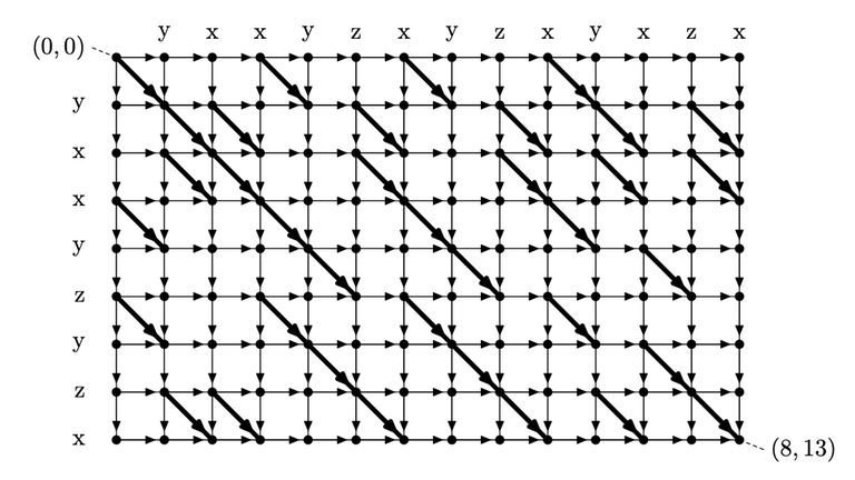
Consider the DP table used in the standard solution of LCS problem. The states and transition form a directed acyclic graph (DAG), and have a shape of a grid graph. Explicitly, the graph consists of:
Figure: DAG constructed from the string "yxxyzyzx", "yxxyzxyzxyxzx"
Here, you can observe that the answer to the query $$$(i, j)$$$ corresponds to the longest path from $$$(0, i-1)$$$ to $$$(N, j)$$$. Let's denote the length of longest path from $$$(x_1, y_1)$$$ to $$$(x_2, y_2)$$$ as $$$dist((x_1, y_1), (x_2, y_2))$$$. Our goal is to compute $$$dist((0, i), (N, j))$$$ for all $$$0 \le i < j \le M$$$.
How can we do this? We need several lemmas:
Lemma 1. $$$dist((0, y), (i, j)) - dist((0, y), (i, j-1))$$$ is either $$$0$$$ or $$$1$$$.
Proof.
Lemma 2. $$$dist((0, y), (i, j)) - dist((0,y ), (i-1, j))$$$ is either $$$0$$$ or $$$1$$$.
Proof. Identical with Lemma 1. $$$\blacksquare$$$
Lemma 3. For every $$$i, j$$$, there exists some integer $$$0 \le i_h(i, j) \le j$$$ such that
Proof. Above statement is equivalent of following: For all $$$y, i, j$$$ we have $$$dist((0, y), (i, j)) - dist((0, y), (i, j-1)) \le dist((0, y+1), (i, j)) - dist((0, y+1), (i, j-1))$$$. Consider two optimal paths from $$$(0, y) \rightarrow (i, j)$$$ and $$$(0, y+1) \rightarrow (i, j-1)$$$. Since the DAG is planar, two paths always intersect. By swapping the destination in the intersection, we obtain two paths $$$(0, y) \rightarrow (i, j-1)$$$ and $$$(0, y + 1) \rightarrow (i, j)$$$ which can not be better than optimal. Therefore we have $$$dist((0, y), (i, j)) + dist((0, y+1), (i, j-1)) \le dist((0, y+1), (i, j)) + dist((0, y), (i, j-1))$$$ which is exactly what we want to prove. $$$\blacksquare$$$
Lemma 4. For every $$$i, j$$$, there exists some integer $$$0 \le i_v(i, j) \le j$$$ such that
Proof. Identical with Lemma 3. $$$\blacksquare$$$
Suppose we have the answer $$$i_h(i, j)$$$ and $$$i_v(i, j)$$$ for all $$$i, j$$$. How can we compute the value $$$dist((0, i), (N, j))$$$? Let's write it down:
$$$dist((0, i), (N, j)) \newline = dist((0, i), (N, i)) + \sum_{k = i+1}^{j} dist((0, i), (N, k)) - dist((0, i), (N, k-1)) \newline = 0 + \sum_{k = i+1}^{j} (i_h(N, k) <= i)$$$
It turns out that we don't even need all values, we only have to know a single linear array $$$i_h(N, *)$$$ ! Given that we have an array $$$i_h(N, *)$$$, the queries can be easily answered in $$$O(\log N)$$$ time with Fenwick trees, or $$$O(1)$$$ time if we use $$$N^2$$$ precomputation.
Hence, all we need to do is to compute the values $$$i_h$$$ and $$$i_v$$$, and it turns out there is a very simple recurrence.
Theorem 5. The following holds:
Proof. Base cases are trivial. For a fixed $$$y$$$, consider the distance from $$$(0, y)$$$ to the four cells in the rectangle $$$(i-1, j-1), (i-1, j), (i, j-1)$$$. Let $$$t = dist((0, y), (i-1, j-1))$$$, then the other two cells either attain value $$$t$$$ or $$$t + 1$$$. Therefore, the possibilities are:
Those three values uniquely determine $$$dist((0, y), (i, j))$$$. You can verify the Theorem 5 by manually inspecting all $$$2^3 = 8$$$ cases by hand. $$$\blacksquare$$$
Remark. At least this is the proof I found, and this is also the proof from the original paper. I believe there is a simpler interpretation, so please add a comment if you have a good idea!
As Theorem 5 gives a simple recurrence to compute all values $$$i_h$$$ and $$$i_v$$$, we can solve the All-Pair LCS problem in $$$O(NM + Q \log N)$$$ time, hence the Range LIS problem in $$$O(N^2 + Q \log N)$$$ time.
As long as SETH Conjecture is true, the longest common subsequence of two strings can not be computed faster than $$$O(NM)$$$ time. Hence our algorithm has no room for improvement. However, in the case of LIS, one of our pattern is fixed as $$$[1, 2, \ldots, N]$$$, and it turns out we can use this to improve the time complexity.
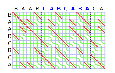
Visualizing the above DP procedure gives a further insight on the structure. We can consider the value $$$i_v$$$ and $$$i_h$$$ to be associated with the edges of the grid: In that sense, the DP transition is about picking the values from the upper/left edges, and routing them to the lower/right edges of the rectangular cell. For example, we can draw a following picture:
In this picture, green curves represent the values — values from the left edges of big rectangle ("BAABCBCA") are $$$0$$$, from the upper edges of big rectangle ("BAABCABCABA") are $$$1, 2, \ldots, M$$$. We will call each green curve as a seaweed. We will also read the seaweed from the lower left corner to the upper right corner, and say the seaweed is in left or right according to this order. In this regard, in the beginning seaweeds are sorted in the increasing order.
Let's reinterpret the DP transition from Theorem 5 with this visualization. If $$$S[i] = T[j]$$$, two seaweed do not intersect. If $$$S[i] \neq T[j]$$$, two seaweed intersect if the right seaweed have a greater value than the left one. In other words, each cell $$$S[i] \neq T[j]$$$ is the anti-sorter of seaweed: If two adjacent seaweeds $$$i, i+1$$$ have increasing values ($$$A[i] < A[i +1]$$$), it swaps so that they have decreasing values ($$$A[i] > A[i+1]$$$).
Of course, in the case of Range LIS we have $$$N^2 - N$$$ such pair, so this is still not enough to solve the problem, but now I can present a main idea for optimization.
Suppose that we swap two values regardless of their values. We can represent each operation as a permutation $$$P$$$ where $$$P(i)$$$ stores the final position of $$$i$$$-th seaweed from the beginning. Let's say we have a swap operation in position $$$i_1, i_2, \ldots, i_k$$$, and let the elementary permutation $$$P_i$$$ be
$$$\begin{equation}P_i(j)=\begin{cases} j+1, & \text{if}\ a=i \newline j-1, & \text{if}\ a=i+1 \newline j, & \text{otherwise}\end{cases} \end{equation}$$$
Then the total operation can be described as a single permutation $$$P = P_{i_1} \circ P_{i_{2}} \circ \ldots \circ P_{i_k}$$$ where $$$P \circ Q$$$ is a composite permutation: $$$P \circ Q(i) = Q(P(i))$$$.
We can't use this to solve the Range LIS problem because we take the values into account. But very surprisingly, even with that condition, there exists a cool operator $$$\boxdot$$$ such that:
The definition of this operator is pretty unintuitive, and needs several auxiliary lemmas:
Definition 6. Given a permutation $$$P$$$ of length $$$N$$$, let $$$\Sigma(P)$$$ be the $$$(N+1) \times (N+1)$$$ square matrix, such that $$$\Sigma(P)_{i, j} = |\{x|x \geq i, P[x] < j\}|$$$
Intuitively, it is a partial sum in left-down direction, for example, if $$$P = [2, 3, 1]$$$, we have:
$$$\Sigma(P) = \begin{bmatrix} 0&1&2&3 \newline 0&1&1&2 \newline 0&1&1&1 \newline 0&0&0&0 \end{bmatrix}$$$
Which is the partial sum of $$$\begin{bmatrix} 0&0&1&0 \newline 0&0&0&1 \newline 0&1&0&0\newline 0&0&0&0 \end{bmatrix}$$$.
Definition 7. Given two matrix $$$A$$$ of size $$$N \times M$$$, $$$B$$$ of size $$$M \times K$$$, the min-plus multiplication $$$A \odot B$$$ is $$$(A \odot B)_{i, j} = min_{1 \le k \le M} (A_{i, k} + B_{k, j})$$$.
Theorem 8. Given two permutation $$$P, Q$$$ of length $$$N$$$, there exists a permutation $$$R$$$ of length $$$N$$$ such that $$$\Sigma(R) = \Sigma(P) \odot \Sigma(Q)$$$. We denote such $$$R$$$ as $$$P \boxdot Q$$$.
To prove it we need two lemmas:
Lemma 8.1. For a matrix $$$\Sigma(R)$$$, there exists a permutation $$$R$$$ if and only if the following conditions are satisfied:
Proof of Lemma 8.1. Consider the inverse operation of partial sums. We can always restore the permutation if the "inverse partial sum" of each row and column contains exactly one $$$1$$$ for each rows and columns, and $$$0$$$ for all other entries. Fifth term guarantees that the elements are nonnegative, third and fourth term guarantees that each rows and columns sums to $$$1$$$. Those conditions are sufficient to guarantee that the inverse yields a permutation. $$$\blacksquare$$$
Lemma 8.2. For any matrix $$$A$$$, $$$A_{i, j} - A_{i, j-1} - A_{i+1, j} + A_{i+1, j-1} \geq 0$$$ for all $$$i, j$$$ if and only if $$$A_{i_1, j_2} - A_{i_1, j_1} - A_{i_2, j_2} + A_{i_2, j_1} \geq 0$$$ for all $$$i_1 \le i_2, j_1 \le j_2$$$.
Proof of Lemma 8.2. $$$\rightarrow$$$ is done by induction. $$$\leftarrow$$$ is trivial. $$$\blacksquare$$$
Proof of Theorem 8. We will prove the first four points of Lemma 9. Note that all entries of $$$\Sigma(R)$$$ are nonnegative since $$$\Sigma(P), \Sigma(Q)$$$ does.
Here, when we consider the derivative, we use the fact that $$$0 \le \Sigma(P)_{i, j} - \Sigma(P)_{i, j - 1} \le 1$$$. $$$N + 1 - j$$$ definitely decreases by $$$1$$$ when we increase the $$$j$$$, but $$$\Sigma(P)_{i, j}$$$ never increases more than $$$1$$$ even when we increase the $$$j$$$. Therefore, it does not hurt to increase the $$$j$$$. We will use this technique later on.
To prove the final point, let $$$k_1, k_2$$$ be the index where $$$\Sigma(R)_{i, j} = \Sigma(P)_{i, k_1} + \Sigma(Q)_{k_1, j}$$$, $$$\Sigma(R)_{i+1, j-1} = \Sigma(P)_{i+1, k_2} + \Sigma(Q)_{k_2, j-1}$$$. Suppose $$$k_1 \le k_2$$$, we have
$$$\Sigma(R)_{i, j-1} + \Sigma(R)_{i+1, j} \newline = \min_k (\Sigma(P)_{i, k} + \Sigma(Q)_{k, j-1}) + \min_k (\Sigma(P)_{i+1, k} + \Sigma(Q)_{k, j}) \newline \le \Sigma(P)_{i, k_1} + \Sigma(P)_{i+1, k_2} + \Sigma(Q)_{k_1, j-1} + \Sigma(Q)_{k_2, j} \newline \le \Sigma(P)_{i, k_1} + \Sigma(P)_{i+1, k_2} + \Sigma(Q)_{k_1, j} + \Sigma(Q)_{k_2, j-1} \newline =\Sigma(R)_{i, j} + \Sigma(R)_{i+1, j-1}$$$
(Note that Lemma 8.2 is used in $$$\Sigma(Q)$$$)
In the case of $$$k_1 \geq k_2$$$ we proceed identically, this time using the Lemma 8.2 for $$$\Sigma(P)$$$. $$$\blacksquare$$$
Theorem 9. The operator $$$\boxdot$$$ is associative.
Proof. Min-plus matrix multiplication is associative just like normal matrix multiplication. $$$\blacksquare$$$
Lemma 10. Let $$$I$$$ be the identity permutation ($$$I(i) = i$$$), we have $$$P \boxdot I = P$$$ (For proof you can consider the derivative.) $$$\blacksquare$$$
And now here comes the final theorem which shows the equivalence of the "Seaweed" and the "Operator":
Theorem 11. Consider the sequence of $$$N$$$ seaweed and sequence of operation $$$i_1, i_2, \ldots, i_k$$$, where each operation denotes the following:
Let $$$P_i$$$ be the elementary permutation as defined above. Let $$$P = P_{i_1} \boxdot P_{i_{2}} \boxdot \ldots \boxdot P_{i_k}$$$ . Then after the end of all operation, $$$i$$$-th seaweed is in the $$$P(i)$$$-th position.
Proof of Theorem 11. We will use induction over $$$k$$$. By induction hypothesis $$$P_{i_1} \boxdot P_{i_{2}} \boxdot \ldots \boxdot P_{i_{k-1}}$$$ correctly denotes the position of seaweeds after $$$k - 1$$$ operations. Let
It suffices to prove that
Which is also equivalent to:
Observe that $$$\Sigma(P_t) - \Sigma(I)$$$ has only one nonzero entry $$$(\Sigma(P_t) - \Sigma(I))_{t+1, t+1} = 1$$$. Since we know $$$\Sigma(A) \odot \Sigma(I) = \Sigma(A)$$$, $$$\Sigma(B)$$$ and $$$\Sigma(A)$$$ only differs in the $$$t+1$$$-th column. For the $$$t + 1$$$-th column, note that
$$$\Sigma(B)_{i, t + 1}$$$ $$$= \min_j (\Sigma(A)_{i, j} + \Sigma(P_t)_{j, t + 1})$$$ $$$= \min(\min_{j \le t} (\Sigma(A)_{i, j} + t + 1 - j), \Sigma(A)_{i, t + 1} + 1, (\min_{j > t+1} \Sigma(A)_{i, j})$$$ $$$= \min(\Sigma(A)_{i, t} + 1,\Sigma(A)_{i, t + 2})$$$ (derivative)
If $$$k_0 < k_1$$$, we have
Which you can verify $$$\Sigma(B)_{i, t+1} = \Sigma(A)_{i, t+1} + 1$$$ iff $$$k_0 < i \le k_1$$$
If $$$k_0 > k_1$$$, we have
Which you can verify $$$\Sigma(B)_{i, t+1} = \Sigma(A)_{i, t+1}$$$ $$$\blacksquare$$$
Yes, this is a complete magic :) If anyone have good intuition for this result, please let me know in comments. (The original paper mention some group theory stuffs, but I have literally zero knowledge on group theory, and I'm also skeptical on how it helps giving intuition)
We learned all the basic theories to tackle the problem, and obtained an algorithm for the Range LIS problem. Using all the facts, we can:
Hence we have... $$$O(N^5 + Q \log N)$$$ time algorithm. Of course this is very slow, but in the next article we will show how to optimize this algorithm to $$$O(N \log^2 N + Q \log N)$$$. We will also briefly discuss the application of this technique.
Yesterday I participated in a local contest involving a problem about Monge arrays. I could've wrote some d&c optimization, but I got bored of typing it so I copypasted maroonrk's SMAWK implementation to solve it. Today, I somehow got curious about the actual algorithm, so here it goes.
I assume that the reader is aware of the concept of D&C Optimization and Monge arrays.
The goal of SMAWK is to compute the row optima (ex. row minima or maxima...) in a $$$n \times m$$$ totally monotone matrix. By totally monotone, it means the following:
Def: Monotone. The matrix is monotone if the position of row optima is non-decreasing.
Def: Totally Monotone (TM). The matrix is totally monotone if every $$$2 \times 2$$$ submatrix is monotone.
Totally monotone matrices are monotone (proof easy but nontrivial), but not vice versa. The latter is a stronger condition. Note that Divide and Conquer Optimization works on a monotone matrix, therefore if you can use SMAWK, you can always use D&C Optimization, but maybe not vice versa. I think it's a niche case, though.
If you want to compute the row minima of a matrix, the TM condition holds iff for all columns $$$p < q$$$:
The takeaway is that if you took $$$(i, q)$$$ as the optimum, then $$$(i + 1, p)$$$ should not be an optimum. At first, I was very confused on the maximum and minimum, but the definition of TM is independent of them. There is absolutely no reason to be confused. On the other hand, sometimes the row optima is non-increasing. You should be careful for that case. The solution is to reverse all rows.
For all columns $$$p < q$$$, if the matrix is TM (per row minima), then if you read columns from top to the bottom you have:
On the other hand, if the matrix is Monge, $$$A[i][p] - A[i][q]$$$ is nondecreasing, therefore:
Basically, SMAWK is a combination of two independent algorithms: Reduce and Interpolate. Let's take a look at both algorithms.
This is the easy one. We can solve $$$n = 1$$$ case naively, so assume $$$n \geq 2$$$. The algorithm works as follows:
For each even rows, we need $$$opt(2k+1) - opt(2k-1) + 1$$$ entries to determine the answer. Summing this, we have $$$T(n, m) = O(n + m) + T(n / 2, m)$$$. This looks ok for $$$n > m$$$, but for $$$n < m$$$ it doesn't look like a good approach.
This is the harder one, but not too hard. Say that we have queries two values $$$A[r][u], A[r][v]$$$ for $$$u < v$$$. Depending on the comparison, you have the following cases:
Let's further proceed with this information. We scan each column from left to right. For each column, we compare it's entries in the first row. We either have
In the second case, we are very lucky — we can remove the whole column! On the other hand, the first case only rules out a single candidate. Let's maintain a stack to maintain all non-useless columns, so we store the first column and move on. If we compare the entries in the second row, we either have
Repeating this, we have the following very simple algorithm:
for (int i = 1; i <= m; i++) {
while (!stk.empty() && A[stk.size()][stk.back()] > A[stk.size()][i])
stk.pop_back();
if (stk.size() < n)
stk.push_back(i);
}
That's it! As a result, we can reduce the number of columns to at most the number of rows in $$$O(n + m)$$$ time.
Now we are ready to present the whole algorithm, and it's so simple:
What is the time complexity? Except for the very first iteration of SMAWK, we can assume that the size of row and column is roughly the same. Then, we spend $$$O(n)$$$ time to halve the size of rows and columns, therefore the time complexity is $$$O(n + m)$$$.
I implemented the above algorithm, which was actually pretty easy: It's not simpler than D&C optimization (since it's very very simple), but I thought it was pretty pleasant to implement. Then I submitted this nice faster linear-time alternatives to the template D&C optimization problems... and got Time Limit Exceeded, because:
Then I just decided to copy-paste maroonrk's SMAWK implementation (I copied it from here), which I'm not sure if it's the fastest, but looks to have some constant optimizations, and was about 2x faster than my implementation. In the online judges, it seemed a little (1.5x?) faster than the D&C optimization for $$$N = 200000$$$.
But it's not faster or simpler than D&C, why should I learn it? I mean, like ad-hoc problems, you don't always do stuff because there is a particular reason to do it, so...
By the way, it is well-known to compute $$$DP[i] = \min_{j} DP[j] + Cost(j + 1, i)$$$ in $$$O(n \log n)$$$ time if the cost is Monge. Normal SMAWK can't optimize this, but it seems there is a variant of SMAWK named LARSCH algorithm which computes this sort of recurrences in $$$O(n)$$$ time. I mean, just so you know...
In today 6pm KST, I will stream solving problems related to Chordal Graphs and Tree decompositions. Stream link is here.
Even if the problem has some special structure, I will ignore it and only assume that it is a Chordal Graph or a graph with bounded treewidth.
Stream will end if someone asks me to play League together. I think it will probably last about 4 hours.
Enjoy!
I recently solved some problems that involved the concept of Lyndon decomposition. Honestly, most of them were too hard to understand for me. I'm just trying to think out loud about things I've read, so I can learn ideas or better takes from smarter people?
Note that I will omit almost all proofs as I can't do that. I believe all unproven claims below are facts, but it is always great to have doubts about anything.
Partly copy-pasted from this link.
A string is called simple (or a Lyndon word), if it is strictly smaller than any of its own nontrivial suffixes. Examples of simple strings are $$$a, b, ab, aab, abb, abcd, abac$$$.
It can be shown that a string is simple, if and only if it is strictly smaller than all its nontrivial cyclic shifts. As a corollary, it can be observed that simple words are never periodic (it is not a repetition of some words for $$$2$$$ or more times).
The Lyndon decomposition of string $$$s$$$ is a factorization $$$s = w_1 w_2 \ldots w_k$$$, where all strings $$$w_i$$$ are simple, and are in non-increasing order $$$w_1 \geq w_2 \geq \ldots \geq w_k$$$.
Alternatively, the Lyndon decomposition of string $$$s$$$ can be represented as $$$s = w_1^{p_1} w_2^{p_2} \ldots w_k^{p_k}$$$. Here, $$$p_i$$$ are positive integers, and $$$w^p_i$$$ denotes the string $$$w$$$ repeated for $$$p_i$$$ times. All strings $$$w_i$$$ are simple, and are in decreasing order $$$w_1 > w_2 > \ldots > w_k$$$. The only difference is that the group of identical factors is grouped as a chunk such as $$$w^p_i$$$.
It is claimed that for any string such a factorization exists and it is unique. However, I can't prove it.
There are two algorithms that compute the Lyndon decomposition in linear time. The first algorithm is the well-known Duval algorithm. E-maxx has a good explanation on this, so I won't discuss it here.
Another algorithm is conceptually much simpler. Given a string $$$S$$$, consider the greedy algorithm that repeatedly removes the smallest suffix from $$$S$$$. By definition, the greedy algorithm always removes a simple word, so the algorithm will return a decomposition consisting of simple words. We believe that the Lyndon decomposition is unique, thus algorithm returns a Lyndon decomposition.
Let's compute the time complexity, the algorithm will iterate at most $$$O(N)$$$ times, and it can find the smallest suffix naively in $$$O(N^2)$$$ time, so the naive implementation will take $$$O(N^3)$$$ time. However, the smallest suffix is just the first entry of the suffix array, so using the fastest suffix array algorithm can optimize each phase to $$$O(N)$$$, giving an $$$O(N^2)$$$ algorithm.
Should we compute the suffix array from scratch in each phase? The removal of a suffix does change the ordering in the suffix array. For example, $$$abac < ac$$$, but $$$aba > a$$$.
However, this issue doesn't apply to our application, where we remove the smallest suffix. Therefore, given a suffix array $$$SA_0, \ldots, SA_{N - 1}$$$ for the string $$$S$$$, one can simply iterate from $$$SA_0$$$ to $$$SA_{N - 1}$$$, and cut the string as long as it is the leftmost position we encountered. As the suffix array can be solved in $$$O(N)$$$, this gives an $$$O(N)$$$ solution to the Lyndon decomposition. I can't prove why this is true. But this looks like a folklore algorithm, so I believe it's true.
For a string of size $$$N$$$, the Lyndon decomposition may have at most $$$O(N)$$$ size, in which case the above algorithms are already optimal. Hence, in this section, we only discuss finding the smallest suffix for each substring in near-constant time, since it may
The removal of a prefix does not change the ordering in the suffix array. To find the smallest suffix in $$$S[x ...]$$$, just find the first entry in the suffix array such that $$$SA_i \geq x$$$.
Duval's algorithm is basically incremental since it repeatedly adds a letter $$$s[j]$$$ to the existing structure. This hints that the Lyndon decomposition can be computed for all prefixes, although it's not entirely straightforward.
I came up with the algorithm to compute all min suffixes for all prefixes. There are other algorithms to compute the min suffixes, such as the one ecnerwala described in this comment.
Duval algorithm maintains a pre-simple string in each iteration. Consider a pre-simple string $$$t = ww\ldots w\overline{w}$$$ for the current prefix. Except for the last string $$$\overline{w}$$$, every other string are simple. And if we take the Lyndon decomposition of $$$\overline{w}$$$, the first element of it is the prefix of $$$\overline{w}$$$, which is obviously less than $$$w$$$. As we know that Lyndon decomposition is unique, we can see that the last element of Lyndon decomposition of $$$\overline{w}$$$ is exactly the smallest suffix of the current prefix.
Thus, the naive algorithm is the following:
However, we don't have to recompute the smallest suffix of $$$\overline{w}$$$ every time. In the decomposition algorithm, we fix the string $$$s_1 = s[0 : i)$$$ and compute the decomposition for the suffix $$$s[i \ldots]$$$. For each relevant $$$i$$$, we use dynamic programming. Let $$$MinSuf[j]$$$ be the length of smallest suffix of $$$S[i \ldots j)$$$ for $$$j > i$$$. If $$$\overline{w}$$$ is empty the smallest suffix is $$$w$$$. Otherwise, since $$$\overline{w}$$$ is exactly the string $$$S[i \ldots i + |\overline{w}|)$$$, $$$MinSuf[j] = MinSuf[i + |\overline{w}|]$$$. Therefore we can obtain a simple recursive formula.
This paper contains some ideas, so if you are interested, give it a try :)
Run is a concept that is useful for solving problems related to repeats. Even if you never heard of the name, anyone who solved some challenging suffix array problems will be familiar with it.
Given a string $$$S$$$, the tuple $$$(l, r, p)$$$ is a run of string $$$S$$$ if
Let $$$-S$$$ be the string where all elements are inverted: Specifically, we assign s[i] = 'a' + 'z' - s[i]
for all elements of $$$S$$$, so that the usual comparison order is reverted, except the empty character which has the lowest priority.
Given a string $$$S$$$, a Lyndon prefix is the longest prefix that is a Lyndon word. Given a suffix array of $$$S$$$, this Lyndon prefix can be easily computed. Recall an algorithm that computes the Lyndon decomposition given a suffix array. Let $$$Rank_i$$$ be the inverse of the suffix array. Then, we can see that the length of the Lyndon prefix is the smallest $$$i$$$ such that $$$Rank_i < Rank_0$$$ (or $$$|S|$$$ if such does not exist). Similarly, we can also compute this for all suffixes $$$S[i \ldots]$$$: find the smallest $$$j > 0$$$ such that $$$Rank_{i + j} < Rank_i$$$.
For each suffix of $$$S$$$ and $$$-S$$$, we compute the Lyndon prefix $$$[i, j)$$$ and take them as a "seed". Start from the tuple $$$(i, j, j - i)$$$, and extend the tuple in both direction as long as $$$S[i] = S[i + p]$$$ holds. Specifically, Let $$$k$$$ be the maximum number such that $$$S[i, i + k) = S[j, j + k)$$$ and $$$l$$$ be the maximum number such that $$$S[i - l, i) = S[j - l, j)$$$. Then we obtain a run $$$(i - l, j + k, j - i)$$$. Both $$$k, l$$$ can be computed in $$$O(\log N)$$$ time with suffix arrays.
It's easy to verify that those elements are actually the run of the string. If we remove all duplicated runs, the following fact holds:
Fact 1. Those we computed are exactly the set of all Runs.
Fact 2. There are at most $$$n$$$ runs.
Fact 3. The sum of $$$(j - i) / p$$$ for all runs are at most $$$3n$$$.
Fact 4. The sum of 2-repeats ($$$j - i - 2p + 1$$$) obtained from runs are at most $$$n \log n$$$.
Fact 3 is useful when we want to enumerate all repeats. Suppose that we have to enumerate all possible repeats. A string "aaaa" can be considered as a repeat of "a" 4 times, but it is also a repeat of "aa" 2 times. In this case, we have to enumerate all multiples of $$$p$$$ — but by Fact 3, that does not affect the overall complexity.
Fact 1, 2, 3 can be found on this paper. I think Fact 4 is not hard to prove, but that doesn't mean I've done it, nor do I have a reference that states this fact.
Given a string $$$S$$$, you can select $$$0$$$ or more non-overlapping substrings, and reverse them. What is the lexicographically minimum result you can obtain from the single iteration of this operation?
Let $$$S^R$$$ be the reverse of $$$S$$$. The answer is to take the Lyndon decomposition for $$$S^R$$$, and reverse each substring from that respective position.
I don't know why this works.
Intuitively, we are replacing each prefix of $$$S$$$ to the minimum suffix of $$$S^R$$$. Replacing each prefix to the minimum possible suffix seems like a good trade. Do you agree or disagree? XD
Given a string $$$S$$$, what is the lexicographically minimum result you can obtain by taking a cyclic shift of $$$S$$$?
The answer can be found by finding the smallest suffix of length $$$> |S|$$$ for string $$$S + S$$$, and rotating at the respective position. This suffix can be found with Lyndon decomposition. Therefore we can solve this in $$$O(n)$$$ time, which is great.
What about just reversing a minimum suffix of $$$S$$$? Unfortunately, cases like "acabab", "dacaba" are the countercase. If we can reduce this problem into a minimum suffix instance, we can solve this problem for all prefixes, suffixes, and possibly substrings, so that's really unfortunate...
.. or maybe not. For a string $$$S$$$, consider it's Lyndon factorization $$$S = w_1^{p_1} w_2^{p_2} w_3^{p_3} \ldots w_k^{p_k}$$$. Clearly, taking the middle of periods is a bad idea. And taking only $$$w_k^{p_k}$$$ as a candidate is wrong.
Then what about trying to crack the tests? Let $$$SFX_j = w_j^{p_j} w_{j+1}^{p_{j + 1}} \ldots w_k^{p_k}$$$. Then, we can try all $$$SFX_j$$$ in range $$$k - 69 \le j \le k + 1$$$ as a candidate. It looks really hard to create an anti-test for this approach.
Lemma. Minimum rotation exists in the last $$$\log_2 |S|$$$ candidates of $$$SFX_j$$$. (Observation 6)
This provides an algorithm for computing the minimum rotation in $$$O(Q(n) \log n)$$$ time, where $$$Q(n)$$$ is time to compute the minimum suffix.
Hello!
XXII Open Cup. Grand Prix of Seoul will be held in 2022/07/17 Sunday, 17:00 KST (UTC+9).
The contest was used as a Day 2 Contest for ByteDance Summer Camp 2022.
Problems were authored by jh05013, molamola., jihoon, ainta, pichulia, chaeyihwan, evenharder, TLEwpdus, applist, Cauchy_Function.
Special thanks to myself for translating the statements and editorials.
Enjoy!
Hello!
XXII Open Cup. Grand Prix of Daejeon will be held in 2022/03/27 Sunday, 17:00 KST (UTC+9). The date of March 27 is final.
Daejeon is home to KAIST, but the contest itself has little to do with it, it just inherits the spirit of 2019 Daejeon GP.
The contest was used as a Day 2 Contest for Petrozavodsk Winter Camp 2022. I'm sorry for the camp participants over the lack of editorial. I will work to publish the full editorials right after the GP.
Problems were authored by ko_osaga, GyojunYoun, tamref, Diuven, queued_q, jh05013. Special thanks to xiaowuc1 for reviewing the statements.
For external accounts, the contest is ready now.
Note that the old opencup.ru link is not accessible now. (snarknews is trying to find servers outside of Russia.)
List of relevant previous contests:
Enjoy!
Update (2021.10.28): Editorial, Division 1 Gym, Division 2 Gym are prepared.
Hello!
XXII Open Cup. Grand Prix of Korea will be held in 2021/10/24 Sunday, 17:00 KST (UTC+9).
For external accounts, the contest is ready now.
List of relevant previous contests:
Enjoy!
Since hmehta didn't wrote anything..
For easy, I spend eternity to realize that every cards starts with their face down. I have so many things to talk about easy, but at this point, it seems worthless.
Will there be a mirror in the near future?
TL;DR: IOI 2021 was planned to held on-site with strong safety measures. Today, IC announced to turn it into an on-line contest (I guess due to travel difficulties). The IC is exploring the possibility of an optional on-site contest.
https://www.facebook.com/ioinformatics.org/posts/458218468862628
Dear Friends of IOI,
I hope you are doing well as COVID-19 is still rampaging all over the world. But as vaccines are becoming available, I hope we can all soon get back to our normal life before the pandemic.
The IC held the Winter meeting in late February. We have the following important information regarding IOI 2021 to share with the community.
First, IOI 2021, organized by Singapore, will still be an online competition much like the previous year. The competition week will fall between mid to late June.
Second, competition aside, in an effort to bring back some normalcy, IOI business will be conducted as usual. This includes collection of registration fees and election of new committee members.
Third, the host and the IC are still exploring possibilities to socially host some teams who can and are willing to travel to Singapore, subject to various Air Travel requirements and COVID-19 safe management measures. Such teams would still sit the contest online from within Singapore, using their own computers. Detailed plans will be announced by the host as they become available.
I hope this information will allow you to start making plans for selecting teams to participate in IOI 2021. The IC and the host team will continue to held online meetings leading up to the IOI in June. We will keep you all updated as things develop further. If you have any questions, please contact the IOI Secretariat at secretary.ioinformatics@gmail.com.
Stay safe and best wishes, Greg Lee IOI President
Hello!
I uploaded 2020 Petrozavodsk Summer Camp, Korean Contest to the CF Gym. It is a collection of Korean problems per the request of snarknews.
Problems are collected from:
Problems are authored by:
And unfortunately there are no editorials.
List of relevant previous contests:
Enjoy!
Название |
---|