Codeforces and Polygon may be unavailable from December 6, 19:00 (UTC) to December 6, 21:00 (UTC) due to technical maintenance. ×

ramchandra's blog

By ramchandra, 4 years ago, In English

Hello everybody,

I've built a function that can be used to display a graph using GraphViz's dot tool. You need to have the dot tool installed or you can copy the graph.dot file to an online dot viewer.

On Ubuntu, this can be installed with the following command: sudo apt install dot

The command works on Linux but will need to be changed on other OSes like Windows. You can copy this function and use it while debugging graph problems.


#include <bits/stdc++.h> using namespace std; void show_graph(const vector<vector<int>> &graph, const bool undirected = true) { /*! Converts graph to dot format *\param undirected is whether graph is undirected or not */ ofstream os{"graph.dot"}; os << (undirected ? "graph" : "digraph"); os << " G {" << endl; for(int u = 0; u < graph.size(); ++u) { for (const auto v : graph[u]) { if (!undirected || u <= v) { os << "\t" << u << (undirected ? " -- " : " -> ") << v << endl; } } } os << "}" << endl; /* Displays dot using image viewer / This command is for Linux. You can change this command for a different OS or for a different image viewer.*/ system("dot -Tpng graph.dot -o graph.png && xdg-open graph.png"); } void add_edge(vector<vector<int>>& graph, const int u, const int v){ /*! Add edge (u, v) to graph*/ graph[u].push_back(v); graph[v].push_back(u); } int main(){ vector<vector<int>> graph(6); add_edge(graph, 1, 2); add_edge(graph, 0, 3); add_edge(graph, 4, 5); add_edge(graph, 0, 5); show_graph(graph, true); }

Dot file produced (graph.dot):


graph G { 0 -- 3 0 -- 5 1 -- 2 4 -- 5 }

The image produced (graph.png):
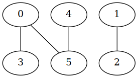
Displayed graph

You can find other useful utilities like this in my template library.

Full text and comments »

  • Vote: I like it
  • +52
  • Vote: I do not like it

By ramchandra, 4 years ago, In English
Introduction

This tutorial is about ear decomposition, a simple but powerful technique for finding graph connectivity, including 2-vertex-connectivity, 2-edge-connectivity, and strong orientation.

In this tutorial we assume we have a connected graph. If the graph is disconnected, the algorithm can be run on each connected component.

An ear consists of a path where the endpoints (the first and last vertices) could be the same or different. So a cycle can be an ear. (It is called an "ear" because it is shaped like the human ear.)

An ear decomposition1 is a decomposition of a graph into a sequence of ears $$$C_1, C_2, \dots, C_n$$$. $$$C_1$$$ must be a cycle and each later ear must be either a path between two vertices that are on previous ears, or a cycle with one vertex on a previous ear.

Since every edge in an ear belongs to a cycle, an ear decomposition has no bridges. So, a connected graph is 2-edge-connected iff it has an ear decomposition containing all its edges.

In an open ear decomposition all ears except the first are paths. A connected graph is 2-vertex-connected iff it has an open ear decomposition containing all its edges. Note that 2-vertex-connectivity implies 2-edge-connectivity.

Finding ear decomposition

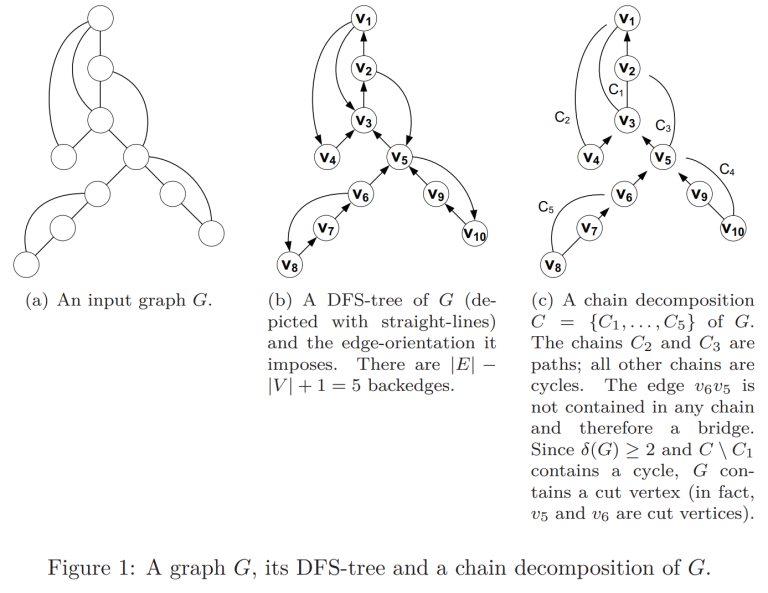
To find an ear decomposition, we use the algorithm in Schmidt (2013b)2. Run a DFS on the graph. Root each edge in the DFS tree towards the root and each backedge away from the root. Note that each edge in a DFS tree is either a backedge between a vertex and its ancestor or a tree edge. For each vertex in DFS order, we loop through each backedge, and traverse the unique directed cycle containing the backedge until we hit a previously visited vertex. The path we traverse is the ear. Note that the first and last vertices of each ear apart from the first one are previously visited. So, if every edge is contained in a ear, we have an ear decomposition of the entire graph, otherwise we have an ear decomposition for a subgraph. The time complexity of this approach is $$$\Theta(|E|+|V|)$$$ since we visit each edge and vertex once.

Example illustration

Source: 2

Finding bridges

A bridge is an edge of the graph whose removal splits the graph into multiple connected components.

The bridges of the graph are exactly the edges that are not in any ear, because the ear decomposition consists of all the edges which are part of a cycle.

Finding articulation points

Analogously, an articulation point is a point of the graph whose removal splits the graph into multiple connected components.

The articulation points are exactly the vertices which are on the endpoint of a cycle apart from $$$C_1$$$ or a bridge.

Strong orientation

A graph has a strong orientation iff the graph has an ear decomposition containing all its edges. To find the strong orientation, we simply orient the graph based on the DFS as described above.

Code:
#include <bits/stdc++.h>
using namespace std;
using ll = long long;
/*! \brief Returns an open ear decomposition of the graph.
* \returns A list of ears for each connected component of the graph is returned.*/
auto ear_decomp(const vector<vector<ll>> &graph) {
    vector<ll> ear_visited(graph.size()), dfs_visited(graph.size()), parent(graph.size());
    vector<vector<vector<ll>>> ears_list;
    for(ll root = 0; root < graph.size(); ++root) {
        if (dfs_visited[root]) {
            continue;
        }
        // Perform a DFS
        vector<ll> queue;
        const auto dfs = [&](const auto& dfs, ll u) -> void {
            dfs_visited[u] = true;
            queue.push_back(u);
            for(const auto v: graph[u]){
                if(dfs_visited[v]){continue;}
                parent[v] = u;
                dfs(dfs, v);
            }
        };
        dfs(dfs, root);
        vector<vector<ll>> ears;
        for (const auto u : queue) {
            for (const auto v : graph[u]) {
                if (parent[u] == v || parent[v] == u) {
                    continue;
                }
                // Found a backedge. Now traverse the ear.
                vector<ll> ear{u};
                ear_visited[u] = true;
                for(ll x = v; ; x = parent[x]){
                    ear.push_back(x);
                    if (ear_visited[x]) {
                        break;
                    }
                    ear_visited[x] = true;
                }
                ears.push_back(ear);
            }
        }
        ears_list.push_back(ears);
    }
    return ears_list;
}
/*! @brief Finds biconnected components of graph using ear decompositions.*/
auto biconnected_ear(const vector<vector<ll>>& graph) {
    // art_points[i] = whether vertex i is an articulation point
    vector<ll> art_points(graph.size());
    // Bridge edges
    vector<array<ll, 2>> bridges;
    // Find ears apart from the first one which are cycles.
    const auto ear_list = ear_decomp(graph);
    for (const auto &ears : ear_list) {
        for(ll i = 0; i < ears.size(); ++i) {
            if (i != 0 && ears[i].front() == ears[i].back()) {
                art_points[ears[i].front()] = 1;
            }
        }
    }
    // Graph containing all ear edges
    vector<vector<ll>> ear_graph(graph.size());
    for (const auto &ears : ear_list) {
        for (const auto &ear : ears) {
            for(ll i = 0; i < ear.size() - 1; ++i) {
                const auto a = ear[i], b = ear[i+1];
                ear_graph[a].push_back(b);
                ear_graph[b].push_back(a);
            }
        }
    }
    // Find edges which are not in ear decomposition
    vector<ll> ear_adj(graph.size());
    for(ll u = 0; u < graph.size(); ++u) {
        vector<ll> non_ear_adj;
        const auto set = [&](const bool val){
            for(const auto v: ear_graph[u]){
                ear_adj[v] = val;
            }
        };
        set(true);
        for(const auto v: graph[u]){
            if(!ear_adj[v]){
                non_ear_adj.push_back(v);
            }
        }
        // Clear ear_adj efficiently
        set(false);
        for (const auto x : non_ear_adj) {
            if (u < x) {
                array<ll, 2> edge{u, x};
                bridges.push_back(edge);
                for(const auto v: edge){
                    if (graph[v].size() > 1) {
                        art_points[v] = true;
                    }
                }
            }
        }
    }
    return {art_points, bridges};
};
Sources:
  1. Ear decomposition
  2. A Simple Test on 2-Vertex- and 2-Edge-Connectivity

Full text and comments »

  • Vote: I like it
  • +168
  • Vote: I do not like it

By ramchandra, 4 years ago, In English

Introduction

The link-cut tree data structure represents a rooted forest (a collection of rooted trees) and can perform the following operations in $$$O(\log n)$$$ amortized time (here, a node represents a vertex of the tree):

  • link(par, child): Attach a tree (child) as a child of another tree's node (par).

  • cut(node): Detach node's subtree from node's parent.

  • find_root(node): Find the root of a node.

  • lca(u, v): Find the least-common ancestor of two nodes.

Structure:

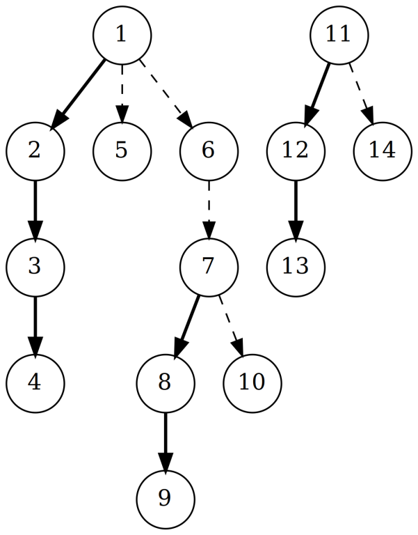
The represented forest (which is represented by the link-cut tree) is split into disjoint, vertical preferred paths composed of preferred edges linking each node with the latest child on the access path. On each preferred path we store a splay tree, sorted by increasing depth. You'll want to know splay trees for link-cut trees so see my splay tree tutorial for a tutorial on splay trees, which are a type of balanced binary search tree. Each preferred path has a path-parent pointer pointing to the root of the parent preferred path (if it exists). So, each edge is either a preferred path edge or path-parent edge.

Diagram:

Link-cut tree

Here, bold edges denote preferred path edges and dashed edges denote path-parent edges. 1 and 11 are the roots of the two trees in the represented forest. The preferred paths are (1,2,3,4), (5), (6), (7, 8, 9), (10), (11, 12, 13), (14).

Avoiding confusion:

Be careful to distinguish the splay tree (the implementation detail) from the represented forest (what we actually care about as a user). Note that the path-parent pointer is different from the splay tree parent pointer. Also note that the root of a tree in the represented forest may not be the splay tree root of the splay tree containing it. Likewise, the splay tree children do not correspond to represented forest children.

Implementation:

Splay tree

Each node will store an additional path parent pointer. Note that since exactly one of the path parent or splay tree parent pointers are null, we can actually store the path-parent pointer in the parent pointer. However, here we choose not to do so, for the sake of simplicity.

The splay tree code must be modified so that the path parent pointer is set to the splay tree parent's path parent pointer.

Splay tree code:


/** @brief Implements a splay tree*/ template<typename T> struct SplayNode{ SplayNode(){} SplayNode(T value_arg): value{value_arg} {} T value{}; //!< Value associated with node array<SplayNode *, 2> child{}; //!< Left and right children SplayNode *parent{}; //!< Pointer to parent Node* path_parent{}; // Added for link-cut tree bool side() const { /*! Returns true if child is on the right, and false otherwise*/ return parent->child[1] == &this; } void rotate() { /*! Rotate node x around its parent */ const auto p = parent; const bool i = side(); if (p->parent) { p->parent->attach(p->side(), &this); } else { parent = nullptr; } p->attach(i, child[!i]); attach(!i, p); this.path_parent = p->path_parent; // Added for link-cut tree } void splay() { /*! Splay node x. x will become the root of the tree*/ for(;parent;rotate()) { if (parent->parent) { (side() == parent->side() ? parent: &this)->rotate(); } } } array<SplayNode *, 2> split() { splay(); // TODO use detach function const auto right = child[1]; if (right) { right->parent = nullptr; } this->right = nullptr; return {&this, right}; } void attach(bool side, SplayNode *const new_) { /*! Attach node new_ as the node's side children*/ if (new_) { new_->parent = &this; } child[side] = new_; } };
Access

The key operation we need is the access(node) operation which moves the node to the root of the splay tree containing the root of the tree containing node in the represented forest. Note that this does not affect the represented forest, but merely reorganizes the internal splay trees and preferred paths. To implement access(node), we splay the node and convert the node's path-parent edge into a splay tree edge (effectively merging the two preferred paths and their splay trees). For implementing access, we use a helper function detach_child which converts a preferred child edge to a path parent edge, effectively splitting the preferred path.

Now we can implement all the other operations in terms of access.

Node *make_tree() {
	/*! Make a new tree */
	return new Node{};
}
void detach_child(Node* node){
	/*! Converts node's preferred child edge to a path parent edge*/
	if(node->child[1]){
		node->child[1]->path_parent = node;
		node->child[1]->parent = nullptr;
	}
}
Node *access(Node *node) {
	/*! Moves node to the root of the auxillary tree containing the root node of the tree. Returns last path-parent of node as it moves up the tree*/
	node->splay();
	detach_child(node);
	node->child[1] = nullptr;
	Node *par = node;
	while (node->path_parent) {
		par = node->path_parent;
		par->splay();
		detach_child(par);
		par->attach(1, node);
		node->path_parent = nullptr;
		node->splay();
	}
	return par;
}
Find root

For find_root(node), we call access(node), and then we find the node with minimum depth in the splay tree containing the (represented forest) root by repeatedly walking to the left child. Since this node has minimum depth, it must be the root. So now node equals the (represented forest) root node. We then access(node) which splays the root to speed up future find_root calls.


Node *find_root(Node *node) { /** Finds the root of the tree containing node*/ access(node); for (; node->child[0]; node = node->child[0]); access(node); return node; }
Cut

For cut, we access the node and then detach it from it's splay tree left child, which is its parent in the represented forest.

void cut(Node *node) {
	/*! Detaches the subtree of node from the tree of node's parent*/
	access(node);
	node->child[0]->parent = nullptr;
	node->child[0] = nullptr;
}
Link

For link(parent, child), we access the child and then access the parent. Then we simply attach the parent as the child's left (splay tree) child.


void link(Node *par, Node *child) { /*! Makes child the child of par*/ access(child); access(par); child->attach(0, par); }

For finding the LCA, we access u, then return the last path-parent of the node (before it becomes the root of the splay tree containing the represent tree's root). This last path-parent node is the node separating the subtree containing u from the subtree containing v.

Node *lca(Node *u, Node *v) {
	/*! Returns lowest common ancestor of nodes u and v or nullptr if u and v are in different trees*/
	if (find_root(u) != find_root(v)) {
		return nullptr;
	}
	access(u);
	return access(v);
}

Obligatory shill comment: my C++ template library OmniTemplate has code for link-cut tree and splay tree (and more).

Uses:

This data structure can be used to speed up Dinic's algorithm from $$$O(V^2 E)$$$ to $$$O(EV\log V)$$$.

You can also augment this with path sums (and other monoid operations) by augmenting the splay tree with sums stored in each node. You can alternatively augment it with subtree sums/size by storing the sum of subtree generated by only considering the path-parent edges in each node and then updating it while performing operations.

Link-cut tree problems:

Full text and comments »

  • Vote: I like it
  • +195
  • Vote: I do not like it

By ramchandra, 4 years ago, In English

This tutorial is about the splay tree, a self-balancing binary search tree.

Key features:
  • $$$O(\log n)$$$ amortized operations.

  • $$$O(n)$$$ construction time complexity (you can simply build a binary search tree)

  • Memory-efficient: no additional space needed apart from the binary search tree.

The key idea behind the splay tree is the splay function, which rotates nodes so as to balance the tree. Since this consists only of tree rotations, this does not affect the binary search tree ordering.

Tree rotation

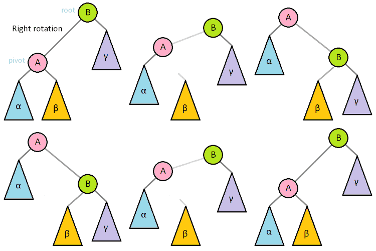
A tree rotation inverts the relationship between a parent and a child node, without affecting the in order traversal of the binary search tree. See the animation below.

Tree rotation

(Animation source: Wikipedia user Tar-Elessar, licensed under CC-BY-SA 4.0)

Splay operation

During a splay step, we repeatedly do this until the node reaches the root: If there is a parent: Rotate the parent if the node's parent is on the same as the node (e.g. the node == node->parent->parent->left->left or node == node->parent->parent->right->right). Otherwise rotate the node. Then rotate the node.

This splay operation tends to balance the tree. The standard BBST operations can be implemented based on splay.

Implementing other operations

To insert a node, insert regularly as you would in a binary search tree (by walking down the binary search tree), and then splay the newly created node. Then set the root node to the newly created node.

To join two splay trees a and b, where all the keys in a are less than all the keys in b, splay the maximum element of a. Since the maximum element of a is now at the root, it has no right child (since it is the maximum element). So, simply attach b as the right child of a. a will then be the joined tree.

To erase a node, splay the node and then join the node's two child subtrees.

Implementation details

Note: you may not want to use recursion in a splay tree as that could lead to stack overflow in the worst-case, where the tree could have depth $$$O(n)$$$. Recursion is alright on Codeforces since it has a large stack limit.

In this implementation, the side function tells us which side the node is relative to its parent. We store the left and right children in an array to simplify the code. That way we can avoid writing two functions rotate_left and rotate_right. Instead, we just need to write one function rotate that handles all the rotation cases. Also, the helper function attach attaches a child node to a parent node. The helper function attach is used.

For finding a node, be sure to splay the last non null node visited to ensure $$$O(\log n)$$$ complexity. (Thanks to Narut for pointing this out)

Applications:

Generally, since they are both BBSTs, splay tree can be used in lieu of treap. So these [treap problems] can be solved with splay tree as well.

Another application is the link-cut tree, a data structure used to represent a rooted forest. Stay tuned for a blog on link-cut tree in a few days.

Code:
#include <bits/stdc++.h>
using namespace std;
using ll = long long int;
/** @brief Implements a splay tree*/
template <typename T> struct SplayTree {
	struct Node {
		Node(){}
		Node(T value_arg): value{value_arg} {}
		T value{}; //!< Value associated with node
		array<Node *, 2> child{}; //!< Left and right children
		Node *parent{}; //!< Pointer to parent
		//Node *path_parent{};
		bool side() const {
			/*! Returns true if child is on the right, and false otherwise*/
			return parent->child[1] == this;
		}
		void rotate() {
			/*! Rotate node x around its parent */
			const auto p = parent;
			const bool i = side();

			if (p->parent) {
				p->parent->attach(p->side(), this);
			} else {
				parent = nullptr;
			}
			p->attach(i, child[!i]);
			attach(!i, p);
		}
		void splay() {
			/*! Splay node x. x will become the root of the tree*/
			for(;parent;rotate()) {
				if (parent->parent) {
					(side() == parent->side() ? parent: this)->rotate();
				}
			}
		}
		array<Node *, 2> split() {
			splay();
			const auto right = child[1];
			if (right) {
				right->parent = nullptr;
			}
			this->right = nullptr;
			return {this, right};
		}
		void attach(bool side, Node *const new_) {
			/*! Attach node new_ as the node's side children*/
			if (new_) {
				new_->parent = this;
			}
			child[side] = new_;
		}
	};
	/** @brief Splay tree node */
	/*! Splay tree iterator */
	struct iterator {
		using iterator_category = bidirectional_iterator_tag;
		using value_type = T;
		using pointer = T *;
		using reference = T &;
		using difference_type = ll;
	      public:
		void operator--() { advance<false>(); }
		void operator++() { advance<true>(); }
		const T &operator*() { return node->value; }
		Node *node;
		iterator(Node *node_arg) : node(node_arg) {}
		bool operator==(const iterator oth) const {
			return node == oth.node;
		}
		bool operator!=(const iterator oth) const {return !(*this == oth);}
	      private:
		template <bool dir> void advance() {
			if (node->child[1]) {
				node = extremum<!dir>(node->child[1]);
				return;
			}
			for (; node->parent && node->side() == dir; node = node->parent)
				;
			node = node->parent;
		}
	};
	Node *root{}; /*!< Root node */
	ll size_{};   /*!< Size of the splay tree*/
	SplayTree() {}
	~SplayTree() { destroy(root); }
	static void destroy(Node *const node) {
		/*! Destroy the subtree node */
		if (!node) {
			return;
		}
		for (Node *const child : node->child) {
			destroy(child);
		}
		delete node;
	}
	void insert(Node *const x) {
		/*! Insert node x into the splay tree*/
		++size_;
		if (!root) {
			root = x;
			return;
		}
		auto y = root;
		while (true) {
			auto &nw = y->child[x->value > y->value];
			if (!nw) {
				nw = x;
				nw->parent = y;
				root = nw;
				nw->splay();
				return;
			}
			y = nw;
		}
		return;
	}
	void insert(const T &key) {
		/*! Insert key key into the splay tree*/
		insert(new Node{key});
	}
	void erase(Node *const x) {
		/*! Erase node x from the splay tree*/
		assert(x);
		x->splay();
		root = join(x->child[0], x->child[1]);
		delete x;
		--size_;
	}
	/** @brief Erases the node with key key from the splay tree */
	void erase(const T &key) { erase(find(key)); }
	template <bool i> static Node *extremum(Node * x) {
		/*! Return the extremum of the subtree x. Minimum if i is false,
		 * maximum if i is true.*/
		assert(x);
		for(; x->child[i]; x = x->child[i]);
		return x;
	}
	static Node *join(Node *const a, Node *const b) {
		if (!a) {
			b->parent = nullptr;
			return b;
		}
		Node *const mx = extremum<true>(a);
		mx->splay();
		assert(mx->child[1] == nullptr);
		mx->child[1] = b;
		mx->parent = nullptr;
		return mx;
	}
    /*! Returns node with key key*/
	Node *find(const T &key) {
		auto x = root;
		while(x && key != x->value){
			const auto next = x->child[key > x->value];
			if(!next){
				x->splay();
			}
			x = next;
		}
		return x;
	}
	/**
     * @brief Returns the number of nodes in the splay tree.
     */
    size_t size() const { return size_; }
	bool empty() const { return size() == 0; }
	iterator begin() { return iterator{extremum<false>(root)}; }
	iterator end() { return iterator{nullptr}; }
};
int main() {
	/*! Tests the splay tree*/
	SplayTree<int> sp;
	sp.insert(4);
	sp.insert(3);
	sp.insert(5);
	assert(sp.size() == 3);
	assert(!sp.empty());
	assert(sp.find(4)->value == 4);
	assert(sp.find(3)->value == 3);
	assert(sp.find(5)->value == 5);
	assert(sp.find(2) == nullptr);
	assert(sp.find(6) == nullptr);
	sp.erase(3);
	assert(sp.size() == 2);
	assert(sp.find(3) == nullptr);
	assert(sp.find(5)->value == 5);
	assert(sp.find(4)->value == 4);
	sp.insert(20);
	sp.insert(-2);
	sp.insert(6);
	vector<ll> expected{-2, 4, 5, 6, 20};
	assert(sp.size() == expected.size());
	for (auto x : expected) {
		assert(sp.find(x)->value == x);
	}
	vector<ll> vec;
	copy(sp.begin(), sp.end(), back_inserter(vec));
	assert(vec == expected);
}

PS: If you liked this code, you can check out my template libary OmniTemplate.

Full text and comments »

  • Vote: I like it
  • +107
  • Vote: I do not like it

By ramchandra, 4 years ago, In English
Introduction

You may have heard of the sparse table data structure, which can do min/gcd queries in $$$O(1)$$$ and sum queries in $$$O(\log n)$$$. The space complexity and time complexity of constructing a sparse table is $$$O(n \log n)$$$.

However, the disjoint sparse table data structure can do any type of query such as sum/min/gcd in $$$O(1)$$$ with the same $$$O(n \log n)$$$ space and time complexity of construction. The operation just needs to be a monoid (i.e. it has an identity element and is associative). Strictly speaking, an identity element is not required, but it allows for empty sum queries which is convenient.

Structure

Here we assume the array is already resized so that its size is a power of $$$2$$$. A disjoint sparse table consists of log n levels numbered from 0 onwards. In the $$$i$$$th level, we split the array into $$$2^i$$$ blocks. For each block, we store the operation sum of elements between any index in the block and the middle of block. For example, level $$$0$$$ would contain one block, whose middle is at $$$mid = n/2$$$, and level $$$1$$$ would contain two blocks, one with middle at $$$n/4$$$ and another with middle at $$$3n/4$$$.

To be specific: if $$$idx < mid$$$, sum[level][idx] stores the sum of elements $$$[idx, mid)$$$, otherwise if $$$idx \geq mid$$$ we store the sum of elements $$$[mid, idx]$$$. In other words, for any given $$$mid = 2^k\cdot o$$$ our table includes all the sums between idx and m for all $$$idx \in [2^k\cdot(o-1), 2^k\cdot(o+1) )$$$. The block with middle $$$mid$$$ has level $$$p-1-k$$$, where $$$n = 2^p$$$.

Since each level contains n elements and there are $$$\log_2 n$$$ levels, the space and time complexity of construction is $$$O(n \log n)$$$

Implementation

To query for the sum of elements in $$$[l,r]$$$, we just need to find the block that includes $$$l$$$ and $$$r$$$.

Suppose we have a disjoint sparse table with $$$7$$$ levels and $$$2^7$$$ elements the binary representation of $$$l$$$ and $$$r$$$ are (using $$$7$$$ bits to represent each index):

$$$l$$$: 1101​[0​]01

$$$r$$$: 1101​[1​]10

Note the leftmost position where the bits differ is at the $$$4$$$th bit (0-indexed) from left marked in square brackets. So, the middle element of block will be $$$1101100$$$. Since the $$$4$$$th bit differs, the level containing this block is $$$4$$$. The range of elements for this block is $$$[1101000, 1101111]$$$. We simply need to add two elements of the table, sum[level][l] which has the sum of $$$[l, mid)$$$ and sum[level][r] which has the sum of $$$[mid, r]$$$.

So, we just need to find the level, which is the position of the leftmost bit that differs. This is simply the leftmost 1 in l^r = 0000111. For finding this we can use the function __builtin_clz(x), a GCC extension that counts the number of leading zeros in the integer $$$x$$$. The functioned is an abbreviation of C​ount L​eading Z​eros. This corresponds to the lzcnt x86 machine instruction, so this is $$$O(1)$$$.

Code
#include <bits/stdc++.h>
using namespace std;
/*! T is the type of the elements
 * Monoid is the operation functor type
 * identity is the identity element of the Monoid (e.g. 0 for addition and inf for minimum)
 */
template <typename T, typename Monoid, auto identity>
class DisjointSparseTable {
public:
	explicit DisjointSparseTable(vector<T> arr) {
		// Find the highest cnt such that pow2 = 2^cnt >= x
		int pow2 = 1, cnt = 0;
		for (; pow2 < arr.size(); pow2 *= 2, ++cnt);
		
		arr.resize(pow2, identity);
		sum.resize(cnt, vector<T>(pow2));
		
		for(int level = 0; level < sum.size(); ++level) {
			for(int block = 0; block < 1 << level; ++block) {
				// The first half of the block contains suffix sums,
				// the second half contains prefix sums
				const auto start = block << (sum.size() - level);
				const auto end = (block + 1) << (sum.size() - level);
				const auto middle = (end + start) / 2;
				
				auto val = arr[middle];
				sum[level][middle] = val;
				for(int x = middle + 1; x < end; ++x) {
					val = Monoid{}(val, arr[x]);
					sum[level][x] = val;
				}
				
				val = arr[middle - 1];
				sum[level][middle - 1] = val;
				for(int x = middle-2; x >= start; --x) {
					val = Monoid{}(val, arr[x]);
					sum[level][x] = val;
				}
			}
		}
	}
	/*! Returns Monoid sum over range [l, r)*/
	T query(int l, int r) const {
		assert(l < r);
		// Convert half open interval to closed interval
		--r;
		if(r == l-1){
			return identity;
		}
		if(l == r){
			return sum.back()[l];
		}
		// Position of the leftmost different bit from the right
		const auto pos_diff = (sizeof(ll) * CHAR_BIT) - 1 - __builtin_clzll(l ^ r);
		const auto level = sum.size() - 1 - pos_diff;
		return Monoid{}(sum[level][l], sum[level][r]);
	}
private:
	vector<vector<T>> sum;
};
int main(){
	// Tests the DisjointSparseTable
	vector<int> data{6, 2, 4, 1, 7, 3, 4, 2, 7, 2, 4, 1, 6};
	DisjointSparseTable<int, plus<>, 0> sp{data};
	for(int start = 0; start < data.size(); ++start) {
		for(int end = start; end <= data.size(); ++end){
			assert(sp.query(start, end) == accumulate(begin(data) + start, begin(data) + end, 0));
		}
	}
}
Credits:

AsleepAdhyyan for telling me about this DS.

I learnt about this DS from Nilesh3105's Disjoint Sparse Table tutorial

EDIT: Fix undefined behavior in calling __builtin_clzll(0) when l == r.

Full text and comments »

  • Vote: I like it
  • +91
  • Vote: I do not like it

By ramchandra, 4 years ago, In English

In this tutorial I'm going to share some useful compilation and debugging tips. These tips can save you a ton of time debugging and make compilation and debugging convenient.

Useful compilation flags

G++ has many useful warning flags such as

  • -Wall enables all warnings. I highly recommend using this flags.
  • -Wextra enables extra warnings.
  • -Wno-sign-conversion silences sign conversion warnings for code like x < vec.size()
  • -Wshadow enables shadowing warnings, so that if you define another variable with the same name in a local scope, you will get a warning.

Using these flags can save you time debugging silly mistakes like forgetting to return a value in a function or doing a comparison like x < vec.size()-1 where vec.size()-1 can underflow into SIZE_MAX-1.

Precompiled headers

You can use precompiled headers to substantially speed up the compilation of your code. Note that the precompiled header is only used if it is compiled with the same flags that your code is compiled with. You can store the precompiled headers in the folder bits/stdc++.h.gch and G++ will automatically find the correct precompiled header (with the correct flags). You can store multiple precompiled headers for bits/stdc++.h for different sets of flags.

sudo g++ -Wall -Wextra -Wshadow -D_GLIBCXX_ASSERTIONS -DDEBUG -ggdb3 -fmax-errors=2 -std=c++17 -o /usr/include/x86_64-linux-gnu/c++/9/bits/stdc++.h{.gch/ASSERT_DEBUG_17.gch,}

Useful debugging flags

Debugging is an important part of CP. After all, even tourist gets RTE on his submissions occasionally.

  • -g enables basic debug information
  • -ggdb3 enables extended debug information such as macros. I suggest using this generally. It slows down compilation a little bit, but has no effect on run-time, since it just adds an extra piece of data in the executable that helps the debugger map the executable file position to line numbers and other related information.
  • -D_GLIBCXX_DEBUG enables out of bounds checking and checks that your comparison operator is irreflexive (comp(a, a) should return false), and many other useful things. However, this can slow down your code runtime (and compile time) substantially.

  • -D_GLIBCXX_ASSERTIONS enables light-weight debug checks such as out of bounds checking. I suggest always using this when compiling locally, as it has negligible runtime and compile-time performance impact.

  • -fmax-errors=<n> limits the number of errors displayed to n. This stops the compiler from printing an excessive amount of error messages.

  • -DDEBUG is used in my debug macro (see below) to enable debugging. Add this to your compilation flags locally to enable debugging. Since this macro is not defined in CodeForces' compilation options, when your code is judged debugging will be disabled.

The _GLIBCXX_* macros are documented in the libstdc++ documentation.

Note that the names of these macros start with an underscore _. The flag -D<macro> defines the macro macro, so you can also use these macros by defining them in the first line before you include any headers.

Example:
#ifdef DEBUG
#define _GLIBCXX_DEBUG
#endif
#include <bits/stdc++.h>
How to use these flags

Add the compilation flag -D_GLIBCXX_DEBUG to define the macro, or likewise -D_GLIBCXX_ASSERTIONS.

Recommended compiler flags

-Wall -Wextra -Wshadow -D_GLIBCXX_ASSERTIONS -DDEBUG -ggdb3 -fmax-errors=2

AddressSanitizer and UndefinedBehaviorSanitizer

The _GLIBCXX_* macros only do debug checks for STL containers and algorithms. So you should use std::array instead of C arrays. For checking for C array out of bounds, use AddressSanitizer with -fsanitize=address. For checking undefined behavior like arithmetic overflow etc use -fsanitize=undefined. You can use them both with -fsanitize=address,undefined.

When upsolving a problem, if you solution does not AC, CodeForces runs sanitizers on it. So you can check the output to see if the sanitizers caught any error.

Debug macro

A useful tool is to have a debug macro that can print useful information like the line number, variable name, etc. Remember to add -DDEBUG to your local compilation flags to enable this debug macro.

#include <bits/stdc++.h>
using namespace std;
// === Debug macro starts here ===

int recur_depth = 0;
#ifdef DEBUG
#define dbg(x) {++recur_depth; auto x_=x; --recur_depth; cerr<<string(recur_depth, '\t')<<"\e[91m"<<__func__<<":"<<__LINE__<<"\t"<<#x<<" = "<<x_<<"\e[39m"<<endl;}
#else
#define dbg(x)
#endif
template<typename Ostream, typename Cont>
typename enable_if<is_same<Ostream,ostream>::value, Ostream&>::type operator<<(Ostream& os,  const Cont& v){
	os<<"[";
	for(auto& x:v){os<<x<<", ";}
	return os<<"]";
}
template<typename Ostream, typename ...Ts>
Ostream& operator<<(Ostream& os,  const pair<Ts...>& p){
	return os<<"{"<<p.first<<", "<<p.second<<"}";
}

// === Debug macro ends here ===

int func(vector<pair<int, string>>& vec){
    dbg(vec);
    return 42;
}
int main(){
    vector<pair<int, string>> vec{{1, "code"}, {2, "forces"}};
    dbg(func(vec));
}

Debug output

Debug output

Note that the debug output is indented based on the recursion level. Also, the output is in red to aid in differentiating debug output from regular output.

Nifty isn't it?

How does the debug macro work?

(you may skip these technical details)

The Ostream template parameter is used so that this operator<< overload has low priority. The operator<< template is also constrained by enable_if so that it does not get called when std::bitset::operator<< is intended to be called.

Debugging using gdb


To debug using gdb, this bash command is useful:

(echo "run < a.in" && cat) | gdb -q a

This automatically runs a with input from a.in.

Quick gdb tutorial

  • start starts your code, pausing execution at main()
  • run runs your code until a breakpoint is hit
  • break <function> pauses execution when a function is called
  • Use up and down to move up and down the stack.
  • jump <line_no> can be used to jump to a line number.
  • continue can be used to continue execution
  • next goes to the next line in the current function
  • step steps into the next line executed (so if you call a function it enters the function's code)
  • You can type abbreviations of these commands, such as r for run.

Adding these flags and commands to ~/.bashrc

If you use the terminal to compile, you can add these functions to your .bashrc file in your home folder (e.g. C:\Users\my_username on Windows). This shell script in this file is executed by bash when you open the terminal. Note that you need to restart your terminal or enter . .bashrc for the changes to take effect.

function compile {
    g++ -Wall -Wextra -Wshadow -D_GLIBCXX_ASSERTIONS -DDEBUG -ggdb3 -fmax-errors=2 -o $1{,.cpp}
}
function debug {
    (echo "run < $1.in" && cat) | gdb -q $1
}

Using these bash functions:

compile a # Compiles a.cpp to a
debug a # Runs a in the debugger with input from a.in

I hope you found this tutorial useful. Feel free to ask any questions or give feedback.

EDIT: Added section on precompiled headers.

Full text and comments »

  • Vote: I like it
  • +208
  • Vote: I do not like it