1 Fast Fourier Transform
1.1 General theory
The fast Fourier transform rests on a key observation:
Theorem (Maschke).
Let $$$G$$$ be a finite group and $$$\Bbbk$$$ a field such that the image of $$$|G|$$$ in $$$\Bbbk$$$ is non-zero.
Then every $$$\Bbbk$$$-representation of $$$G$$$ is semisimple.
Proof.
Because $$$\Bbbk$$$ is a field, it suffices to show that every subrepresentation is a direct summand.
Let $$$V$$$ be a representation of $$$G$$$ and $$$U\subseteq V$$$ a subrepresentation.
Choose a (linear) projection $$$\pi:V\to U$$$.
Average it:
One checks that $$$\tau$$$ is a $$$\Bbbk$$$-homomorphism, hence $$$\ker\tau$$$ is a subrepresentation of $$$V$$$ and $$$U$$$ is a direct summand of $$$V$$$.
Corollary.
Let $$$G$$$, $$$\Bbbk$$$ be as above and let $$${U_i}$$$ be the irreducible representations of $$$G$$$. Then
Proof.
The group algebra $$$\Bbbk[G]$$$ carries the regular representation $$$G\to\mathrm{End}_{\Bbbk}\Bbbk[G]$$$.
All irreducible representations occur in $$$\Bbbk[G]$$$, and by semisimplicity the regular representation is their direct sum. Thus
and comparing dimensions gives the claim.
Hence, replacing an element $$$x\in\Bbbk[G]$$$ by its values on all irreducible representations lowers the complexity of multiplication in $$$\Bbbk[G]$$$ from $$$\Theta(|G|^2)$$$ to
This replacement is the Fourier transform, written $$$x\mapsto\hat x$$$.
A naïve Fourier transform costs $$$\Theta(|G|^2)$$$, so we look for faster ways.
For a function $$$f:G\to\Bbbk$$$ define
and its inverse transform by
where $$$\mathcal R$$$ is a complete set of irreducibles and $$$d_\rho=\dim V_\rho$$$.
Take a subgroup $$$H\le G$$$ and a set of coset representatives $$$C={s_i}$$$. Then
However $$$\rho|_H$$$ need not be irreducible, so we block-diagonalise $$$\widehat x_{\rho|_H}$$$ with a suitable basis $$$\mathfrak B$$$; for concrete groups we construct $$$\mathfrak B$$$ explicitly.
The running time satisfies
After a little manipulation,
Because $$$\dim\rho\le\sqrt{|G|}$$$ one gets
Theorem (Lev).
Unless $$$G\simeq\Bbb Z/p\Bbb Z$$$, the group $$$G$$$ has a proper subgroup of order at least $$$\sqrt{|G|}$$$.
Proof.
Lev’s proof uses the classification of finite simple groups, and we omit it.
Taking $$$|H|=\sqrt{|G|}$$$ yields
This beats the trivial bound only if $$$\omega\le\frac83$$$.
In practice $$$|H|=\sqrt{|G|}$$$ is too large.
If every subgroup $$$H$$$ of $$$G$$$ has a proper subgroup of size $$$|H|^\theta$$$, then
With $$$\omega=3$$$ this is advantageous once $$$\theta\ge\frac23$$$, which is typical for most groups.
1.2 Generic fast Fourier transform
Assume $$$\Bbbk$$$ is algebraically closed of characteristic 0 (or large enough).
If $$$G$$$ embeds in $$$\Bbbk^\times$$$, all irreducible representations are one-dimensional.
For $$$G=\Bbb Z/n\Bbb Z$$$ one has
by the Chinese remainder theorem.
Since every representation is 1-dimensional, restrictions stay irreducible, so no basis change is needed.
Thus
For $$$G=\Bbb Z/n\Bbb Z$$$ and the character $$$\rho(g)=e^{2\pi i g /n}$$$,
and the cost obeys
In practice one works in $$$\Bbbk[X]\bmod(X^n-1)$$$, embeds $$$\Bbbk$$$ in a large $$$\Bbb Z/N\Bbb Z$$$ with $$$N \gt 2n$$$, often taking $$$N=2^k$$$, giving
the classical fast Fourier transform.
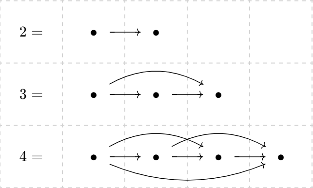
For $$$N=2^k$$$ let $$$x=x_{k-1}\dots x_1x_0$$$ be the binary expansion of $$$x\in\Bbb Z/N\Bbb Z$$$.
Rewrite
so the processing order is
Swapping the $$$x$$$-th and $$$\operatorname{rev}(x)$$$-th values and then performing butterflies for each $$$0\le j \lt k$$$ yields the radix-2 FFT.
1.3 Fast Fourier transform over small-characteristic finite fields
When $$$p-1$$$ is smooth, Section 1.2 suffices.
We now outline the additive Fourier transform on $$$\Bbb F_{p^{p^k}}$$$ due to Cantor and successors.
Write $$$\mathbb K=\Bbb F_{p^{p^k}}$$$, $$$\mathbb F=\Bbb F_p$$$.
Definition.
The canonical $$$\mathbb F$$$-linear map $$$\wp:\mathbb K\to\mathbb K$$$, $$$\wp(x)=x^p-x$$$, is the Artin–Schreier map.
Its $$$i$$$-fold composition is $$$s_i$$$.
Proposition.
The zero set of $$$s_i$$$ is an $$$\mathbb F$$$-vector space.
It is a subfield of $$$\mathbb K$$$ iff $$$i=p^j$$$.
Proof.
Linearity is clear.
If $$$i=p^j$$$, then $$$s_i(x)=x^{p^i}-x$$$ and $$$\mathbb K$$$ contains exactly one subfield of size $$$p^{p^j}$$$; conversely only these $$$i$$$ give subfields.
Set $$$W_i=\ker s_i$$$.
For a polynomial $$$p$$$ of degree $$$ \lt p^i$$$, its additive Fourier transform $$$\mathcal A(p)$$$ is the list of values $$$p(\omega)$$$ with $$$\omega\in W_i$$$ in a fixed order.
Definition.
A Cantor generator sequence $$${g_j}$$$ satisfies
where $$$\deg f \lt i(p-1)$$$ and $$$g_i$$$ has no term of degree $$$\ge p$$$.
It yields the Cantor basis
Theorem.
There is $$$\lambda\in\mathbb F$$$ such that $$$s_j(b_k)-\lambda b_{k-j}\in W_{k-j}$$$.
In particular $$$s_k(b_k)=1$$$ and $$$W_k=\mathrm{span}{b_0,\dots,b_{k-1}}$$$.
Cantor constructs generators with $$$\wp(g_0)=0$$$ and
$$$\wp(g_{k+1})=g_k^{\,M}$$$, where
This gives a Cantor basis and a degree-$$$p^k$$$ irreducible polynomial.
Using the basis $$$X_i$$$ obtained from the $$$g_k$$$, Cantor shows how to convert between the coefficients of a degree $$$ \lt p^D$$$ polynomial and its coordinates in the $$$X_i$$$ basis in
versus the naïve $$$\Theta(D^2p^D\mathrm{poly}(p))$$$.
With this, one derives a divide-and-conquer additive FFT similar to the classical case.
For instance FFTs in the Nim-product field $$$\Bbb F_{2^{64}}$$$ often use Cantor’s method.
1.4 Frobenius-accelerated Fourier transform
Let $$$\sigma:\alpha\mapsto\alpha^{p^m}$$$ be the $$$m$$$-th Frobenius automorphism.
Two elements $$$\alpha,\beta\in\mathbb K$$$ are conjugate if $$$\sigma(\alpha)=\beta$$$ for some $$$\sigma\in\mathrm{Gal}(\mathbb K/\mathbb F)$$$.
Proposition.
If $$$\alpha\in W_k\setminus W_{k-1}$$$, the number of conjugates of $$$\alpha$$$ is $$$p^{\lceil\log_p k\rceil}$$$.
Proof.
$$$\mathbb F(\alpha)=\mathbb F(g_0,\dots,g_{\lceil\log_p k\rceil-1})$$$, so the stabiliser of $$$\alpha$$$ is generated by the $$$p^{\lceil\log_p k\rceil}$$$-th Frobenius; orbit-stabiliser finishes the count.
These conjugates are reached by Frobenius maps of orders $$$p^0,\dots,p^{\lceil\log_pk\rceil-1}$$$, each modifying a specific coordinate in the Cantor basis.
Thus one representative set is
Computing the transform only for $$$\Sigma$$$ and propagating the result along Frobenius orbits reduces time by roughly a factor $$$p/d$$$ with $$$d=\lceil\log_p n\rceil$$$.
See the paper arXiv:1802.03932 and the linked code repository for details; the original idea appears in the “Frobenius FFT” paper cited.
For $$$\Bbb F_{2^{64}}$$$ with Cantor basis $$$1,2,4,8,\dots$$$, the Cantor and Frobenius FFTs give efficient Nim-product multiplication.
1.5 Arbitrary rings
Cantor also devised a fast multiplication algorithm over a general ring $$$R$$$ (associativity can even be dropped).
Fix a radix $$$s=\Theta(1)$$$.
We would like division and roots of unity; instead we avoid division and adjoin roots.
In the Fourier inversion formula the only division is by $$$n=s^r$$$.
For polynomials $$$A,B\in R[X]/(X^n-1)$$$ we can compute $$$n \cdot [X^k]\, (A \cdot B)$$$ as follows: write $$$c$$$ for the $$$k$$$-th coefficient and $$$c'$$$ for the carry from degree $$$k+n$$$.
Running the FFT twice, once at $$$\omega_{ns}$$$ and once at $$$\omega_{ns}\cdot\omega_s$$$, gives $$$n(c+c')$$$ and $$$n(c+\omega_sc')$$$.
Solving the two linear equations needs only ring operations provided some $$$\chi\in R$$$ satisfies $$$(1-\omega_s)\chi\in\Bbb Z\setminus{0}$$$; the limit
shows such a $$$\chi$$$ exists.
Hence we recover $$$c$$$ by Bézout’s identity.
To obtain roots of unity we extend $$$R$$$ to $$$\overline R=R[\omega_n]=R[X]/(\Phi_n)$$$.
Multiplication by $$$\omega_n$$$ becomes a cyclic shift, so DFT uses only additions and shifts.
Recursively multiplying the auxiliary integers yields
Another classic of this flavour is the Toom–Cook method, which evaluates at $$$2k+1$$$ points and satisfies
1.6 Symmetric groups
We quote the structure theorem for irreducibles of $$$S_n$$$ without proof.
Write a Young diagram as a sequence $$$r_1\ge\dots\ge r_n$$$ and a Young tableau by filling it with numbers.
For a tableau let $$$c(i)$$$ be the row index minus column index of the entry $$$i$$$.
Theorem.
Let $$$\lambda$$$ be a Young diagram and $$$\rho_\lambda$$$ its irreducible representation.
For the transposition $$$\sigma=(k\;k+1)$$$ the matrix $$$\rho_\lambda(\sigma)$$$ has rows and columns indexed by standard tableaux of shape $$$\lambda$$$.
Set $$$R=1$$$ if applying $$$\sigma$$$ to tableau $$$t$$$ gives another standard tableau and $$$R=0$$$ otherwise. Then
Clausen designed an FFT for $$$S_n$$$.
He maps $$$\sigma\in S_n$$$ to the permutation obtained by deleting $$$n$$$; in cycle notation this is $$$(\sigma_n\;\sigma_{n+1}\;\dots\;n)$$$.
In the general algorithm of 1.1 one needs a basis in which restriction from $$$S_n$$$ to $$$S_{n-1}$$$ becomes block diagonal.
Clausen observed that this basis is inherited, i.e. the change-of-basis matrix $$$P$$$ is the identity.
Sketch.
A node $$$n$$$ can occupy only those cells whose right and bottom neighbours are empty.
All tableaux with $$$n$$$ in the same position form a class.
For $$$\sigma\in S_{n-1}$$$ the position of $$$n$$$ stays fixed, so $$$\rho_\lambda(\sigma)$$$ is block diagonal, each block being an irreducible of $$$S_{n-1}$$$.
For sparse inputs one may shrink the domain via double cosets such as
gaining freedom to handle parts without FFT.
The library $$$\mathbb S_n\text{ob}$$$ is a classic implementation; see also $$$\mathbb S_n\text{FFT}$$$ for machine-learning applications.
Regarding preference rankings encoded as permutations, define the acceptance between $$$\sigma,\tau$$$ by
let $$$f_\sigma$$$ be the corresponding vector in $$$\Bbb R^{n!}$$$, and consider the clustering problem of partitioning $$$m$$$ such rankings into $$$k$$$ classes minimising
Using Parseval on finite groups:
Theorem (Parseval).
For $$$f:G\to\Bbb C$$$ and unitary irreducibles $$$\mathcal R$$$,
where $$$|\cdot|_{\mathrm{HS}}$$$ is the Hilbert–Schmidt norm.
Proof.
By Peter–Weyl, $$$L^2(G)$$$ splits orthogonally into $$$\sqrt{d_\pi}\,\pi$$$.
Writing $$$f$$$ in this basis and computing coefficients gives
hence
Thus the clustering objective equals
and in practice only a few $\pi$’s suffice for a good approximation, making the computation faster.