


Introduction
For those who have studied the Inclusion-Exclusion Principle or the Mobius Inversion formula, you may have wondered about the definition of $$$μ(n)$$$ and the process of offsetting unnecessary values by multiplying $$$(-1)^{|s|}$$$. Although it is possible to show the validity of these formulas through expansion, such proofs lack intuitive clarity.
In this article, I will define Zeta and Mobius Transform on a Poset and explore examples from various Posets. Understanding these concepts will provide insights into the Inclusion-Exclusion Principle and the Mobius Inversion formula. Additionally, Zeta and Mobius Transform are essential concepts connected to SOS DP and AND, OR, GCD, LCM Convolution. In the final part of the article, we will examine interesting connections to various convolutions from Zeta and Mobius Transform.
Table of Contents
- What is Poset?
- Zeta, Mobius Transform on Poset ($$$ζ$$$ ↔ $$$μ$$$)
- Definition of Mobius function ($$$μ(s, t)$$$)
- Examples
- Fast Zeta, Mobius Transform
- $$$ζ$$$ → convolution → $$$μ$$$
1. What is Poset?
A Poset ($$$S$$$, $$$≤$$$) is a set $$$S$$$ with a relation $$$≤$$$ that satisfies the following properties.
- Reflexive: For all $$$s ∈ S$$$, $$$s ≤ s$$$.
- Antisymmetric: If $$$a ≤ b$$$ and $$$b ≤ a$$$, then $$$a = b$$$.
- Transitive: If $$$a ≤ b$$$ and $$$b ≤ c$$$, then $$$a ≤ c$$$.
There may be pairs of $$$a, b ∈ S$$$ for which the $$$≤$$$ operator is not defined. For example, in $$$S = \lbrace a, b, c \rbrace$$$, although $$$a ≤ b$$$ and $$$a ≤ c$$$ hold, there might be no defined relationship between $$$b$$$ and $$$c$$$. For this reason, ($$$S$$$, $$$≤$$$) is referred to as a Partially Ordered Set (Poset).
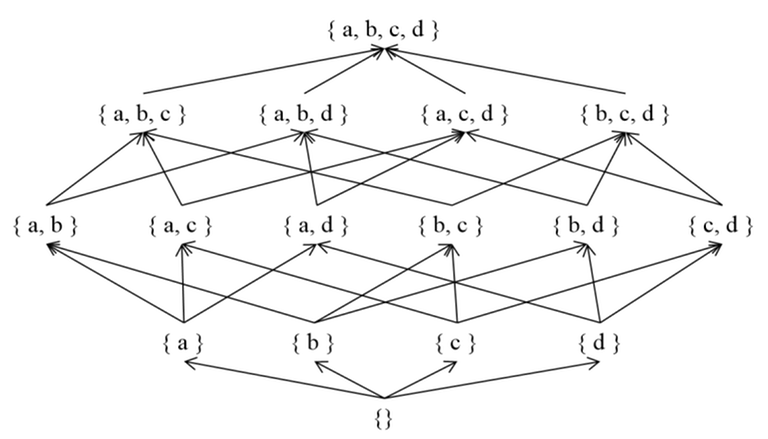
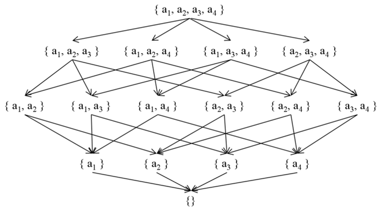
Posets can be effectively visualized using Directed Acyclic Graphs (DAG). Placing the elements of $$$S$$$ as vertices and representing $$$(a, b)$$$ pairs where $$$a, b ∈ S$$$ and $$$a ≤ b$$$ as edges $$$a → b$$$, we can obtain a DAG. To simplify the visualization, we exclude self-loops ($$$a$$$ → $$$a$$$) and redundant edges (e.g., $$$a$$$ → $$$c$$$ when $$$a$$$ → $$$b$$$ and $$$b$$$ → $$$c$$$ are present) and create a Hasse Diagram, which succinctly represents the $$$≤$$$ relationship between elements.
In the upcoming sections, the descendant relationship of vertices will be crucial for the Zeta and Mobius Transform. A vertex $$$a$$$ is considered a descendant of $$$b$$$ if there exists a path from $$$b$$$ to $$$a$$$.
2. Zeta, Mobius Transform on Poset ($$$ζ$$$ ↔ $$$μ$$$)
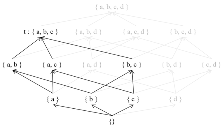
In a Poset ($$$S$$$, $$$≤$$$), let's define $$$g(t)$$$ as follows.
Here, $$$g(t)$$$ is defined as the sum of $$$f(s)$$$ for all $$$s$$$ such that $$$s ≤ t$$$. In other words, $$$g(t)$$$ represents the sum of $$$f$$$ values for the descendants of $$$t$$$. For instance, $$$g(\lbrace a, b \rbrace)$$$ is equal to $$$f(\lbrace a, b \rbrace) + f(\lbrace a \rbrace) + f(\lbrace b \rbrace) + f(\lbrace \rbrace)$$$. To simplify, we can define $$$ζ(s, t)$$$ as $$$1$$$ if $$$s ≤ t$$$ and $$$0$$$ otherwise, allowing us to remove the condition $$$s ≤ t$$$ from the summation expression.
This process of obtaining $$$g$$$ values from the given $$$f$$$ values is called the Zeta Transform.
Now, we want to find an appropriate $$$μ$$$ function that satisfies the above equation and enables us to reconstruct the values of $$$f$$$ from the given $$$g$$$ values.
The process of obtaining $$$f$$$ values from the given $$$g$$$ values is called the Mobius Transform.
3. Definition of Mobius function ($$$μ(s, t)$$$)
The function $$$μ(s, t)$$$ can be defined recursively as follows.
Let's understand the significance of the $$$μ$$$ function's definition in the context of a Poset's DAG.
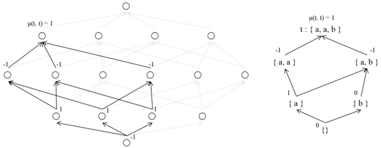
Starting from $$$t$$$ and moving along the backward edges in topological order, let's determine $$$μ(s, t)$$$ for each $$$s$$$. The value of $$$μ(t, t)$$$ is $$$1$$$. For $$$s ≠ t$$$, we can calculate the value of $$$μ(s, t)$$$ such that for $$$s \lt u \leq t$$$, which represents ancestors of $$$s$$$ and descendants of $$$t$$$, we find the sum of $$$μ(u, t)$$$ and multiply it by $$$-1$$$.
By the definition, the $$$μ$$$ function has the property that sum of all $$$μ(u, t)$$$ for all $$$s ≤ u ≤ t$$$ equals $$$1$$$ only if $$$s = t$$$; otherwise, it is always $$$0$$$. From a DAG perspective, if we fix $$$t$$$ and select an arbitrary descendant $$$s$$$ of $$$t$$$ which is not $$$t$$$, the sum of all $$$μ(*, t)$$$ values between $$$s$$$ and $$$t$$$ will always be $$$0$$$. This property is essential to the $$$μ$$$ function and allows it to be used in the Mobius Transform.
Now, let's prove the validity of the Mobius Transform equation.
By expressing the property of the $$$μ$$$ function using the $$$ζ$$$ function, the sum of $$$ζ(s, u) μ(u, t)$$$ is equal to $$$[s = t]$$$. Here, $$$[s = t]$$$ represents the Iverson bracket, which evaluates to $$$1$$$ if the inner statement is true and $$$0$$$ otherwise.
After expanding the Mobius Transform equation, we can use the above property to show the contribution of $$$f(s)$$$ to the entire equation is $$$[s = t]$$$. The variable $$$f(s)$$$ appears once for each $$$g(u)$$$ where $$$s ≤ u$$$, and $$$g(u)$$$ is multiplied by $$$μ(u, t)$$$ before being added to the overall equation. The contribution of $$$f(s)$$$ in the entire equation depends on the sum of $$$μ(u, t)$$$ for $$$s ≤ u ≤ t$$$. Through the previous discussion, we know that this contribution is $$$1$$$ only when $$$s = t$$$. ■
Therefore, the $$$μ$$$ function is suitable for the Mobius Transform.
4. Examples
The method to calculate $$$μ(s, t)$$$ in a Poset ($$$S$$$, $$$≤$$$) can vary depending on how $$$S$$$ and $$$≤$$$ are defined.
In this section, we will calculate $$$μ(s, t)$$$ in various ($$$S$$$, $$$≤$$$) definitions and find the Zeta and Mobius Transform formulas.
1. When $$$S$$$ is a set and $$$≤$$$ is the subset relation
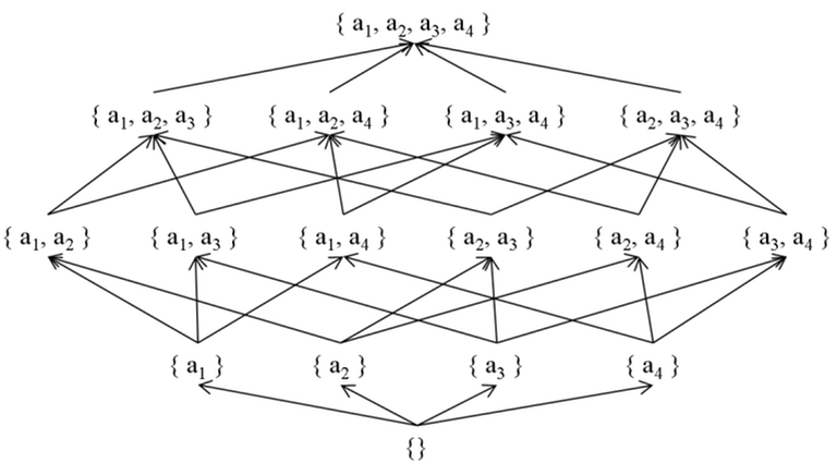
Using the definition of $$$μ(s, t)$$$, for $$$s ⊆ t$$$, $$$μ(s, t)$$$ is $$$(-1)^{|t \setminus s|}$$$.
Proof: The proof begins with the base case where $$$t = ∅$$$, and then uses mathematical induction on $$$|t \setminus s|$$$. Let $$$|t \setminus u| = i$$$ where $$$u$$$ is ancestor of $$$s$$$ and descendant of $$$t$$$. The number of such $$$u$$$ is $$$_{|t \setminus s|}C_{i}$$$. Assuming that $$$μ(u, t) = (-1)^{|t \setminus u|}$$$, we find that $$$μ(s, t)$$$ is equal to $$$-\sum_{i=0}^{|t \setminus s| - 1}{(-1)^i _{|t \setminus s|} C _{i}}$$$. Using the binomial theorem and simplifying the expression, we obtain $$$μ(s, t) = (-1)^{|t \setminus s|}$$$. ■
$$$g(t)$$$ can be obtained by iterating over the subsets $$$s$$$ of $$$t$$$ and adding $$$f(s)$$$, and $$$f(t)$$$ can be obtained by iterating over the subsets $$$s$$$ of $$$t$$$ and adding $$$(-1)^{|t \setminus s|} g(s)$$$.
2. When $$$S$$$ is a set and $$$≤$$$ is the superset relation
In this case, $$$≤$$$ is $$$⊇$$$ (superset) instead of $$$⊆$$$ (subset). Since the direction of the relation is reversed, the Hasse Diagram corresponding to the Poset also has its edges reversed.
For two Posets where the relations are opposite, $$$ζ$$$ and $$$μ$$$ functions in the original Poset can be related to $$$ζ$$$, $$$μ$$$ functions in the transformed Poset as follows: $$$ζ'(s, t) = ζ(t, s)$$$ and $$$μ'(s, t) = μ(t, s)$$$.
Proof: The proof is trivial for the $$$ζ$$$ function. For the $$$μ$$$ function, we can use the fact that $$$\sum_{s \leq u \leq t}{μ(u, t)} = [s = t]$$$ is equivalent to the definition of $$$μ(s, t)$$$. Using this, showing $$$\sum_{s \leq u \leq t}{μ(s, u)} = [s = t]$$$ is enough. Treating $$$ζ(i, j)$$$ and $$$μ(i, j)$$$ as elements of a matrix, we have $$$\sum_{k}ζ(i, k) μ(k, j) = [i = j]$$$, which implies that $$$ζ$$$ and $$$μ$$$ are inverse matrices. From $$$ζ μ = μ ζ = I$$$, we can also deduce $$$\sum_{k}μ(i, k) ζ(k, j) = [i = j]$$$, so the sum of $$$μ(s, u)$$$ for $$$u$$$ where $$$s ≤ u ≤ t$$$ is $$$[s = t]$$$. ■
Therefore, for $$$t ⊇ s$$$, $$$μ(t, s)$$$ is $$$(-1)^{|t \setminus s|}$$$.
$$$g(s)$$$ can be obtained by iterating over the supersets $$$t$$$ of $$$s$$$ and adding $$$f(t)$$$, and $$$f(s)$$$ can be obtained by iterating over the supersets $$$t$$$ of $$$s$$$ and adding $$$(-1)^{|t \setminus s|} g(t)$$$.
Problem: https://www.acmicpc.net/problem/17436
Solution: http://boj.kr/02f08c67d80a4e28aa5847e1fa0c05cb
3. When $$$S$$$ is $$$ℕ$$$ (natural numbers) and $$$≤$$$ is the divisor relation
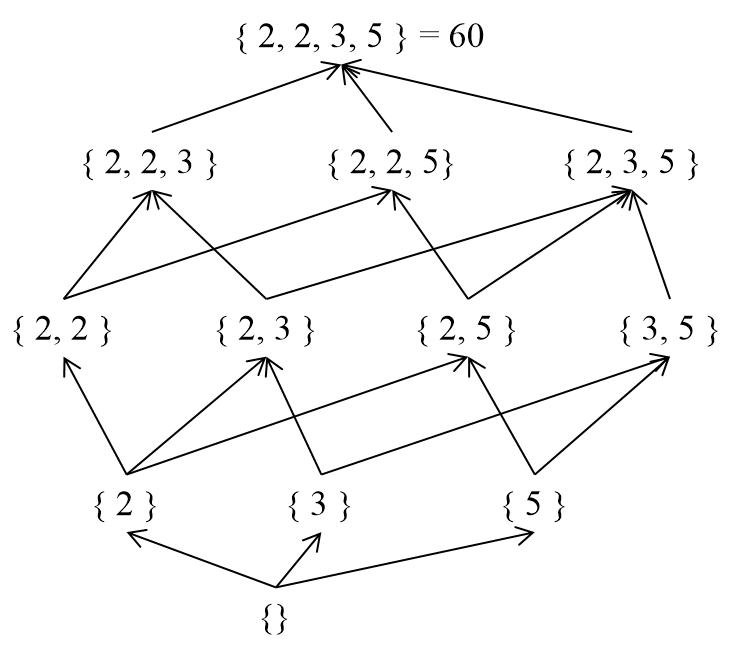
In this case, when $$$d | n$$$, $$$μ(d, n)$$$ is equal to $$$μ(n / d)$$$. Here, $$$μ(x)$$$ is the Mobius function in number theory. If $$$x$$$ has no square factors, then $$$μ(x)$$$ is equal to $$$(-1)^k$$$, where $$$k$$$ is the number of prime factors of $$$x$$$. Otherwise, $$$μ(x)$$$ is $$$0$$$.
(Reference: https://en.wikipedia.org/wiki/M%C3%B6bius_function)
Proof: We can represent $$$n$$$ as $$$p_1^{e_1} ... p_k^{e_k}$$$, and view it as a multiset $$$\lbrace p_1, ..., p_1, ..., p_k, ..., p_k \rbrace$$$ (with $$$p_i$$$ occurring $$$e_i$$$ times). We can then consider the relation $$$d | n$$$ (meaning $$$n$$$ is divisible by $$$d$$$) as a $$$⊆$$$ relation on the set. We will apply mathematical induction on $$$n$$$. When $$$d | n$$$, $$$μ(d, n)$$$ can be expressed as $$$-\sum_{d | d' | n, d \lt d'} μ(d', n)$$$. First, let's consider the case where the multiset of $$$n / d$$$ has no duplicate elements. By assuming that $$$μ(d', n)$$$ is $$$μ(n / d')$$$, we find that $$$μ(d', n) = (-1)^i$$$, where $$$i$$$ is the number of prime factors of $$$n / d'$$$. There are $$$_iC_k$$$ multisets where k is the number of prime factors of $$$n / d$$$, so $$$μ(d, n) = -\sum_{i=0}^{k-1} {_kC_i (-1)^i} = -((1 - 1)^k - (-1)^k) = (-1)^k = μ(n / d)$$$. If the multiset of $$$n / d$$$ contains duplicate elements, we can consider the multiset $$$s$$$ obtained by removing the duplicate elements. For any $$$s' ⊆ s$$$, the sum of the $$$μ$$$ values of $$$s'$$$ is $$$0$$$, so $$$μ(d, n) = 0 = μ(n / d)$$$. ■
$$$g(n)$$$ can be obtained by iterating over the divisors $$$d$$$ of $$$n$$$ and adding $$$f(d)$$$, and $$$f(n)$$$ can be obtained by iterating over the divisors $$$d$$$ of $$$n$$$ and adding $$$μ(n / d) g(d)$$$.
4. When $$$S$$$ is $$$ℕ$$$ (natural numbers) and $$$≤$$$ is the multiple relation
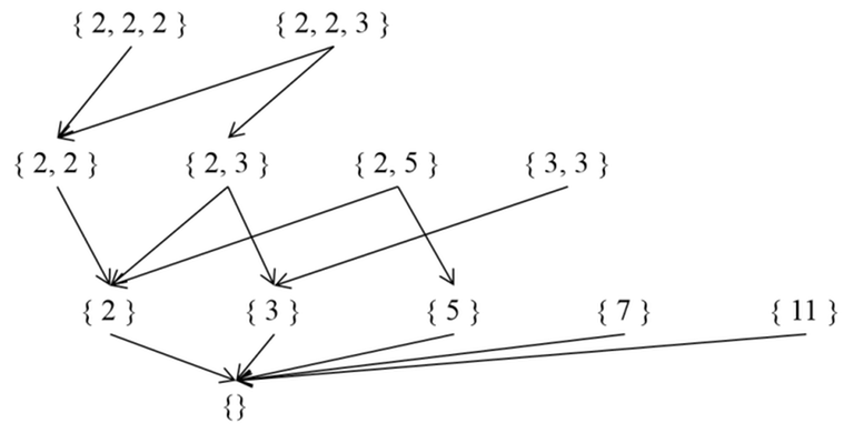
In this case, the relation is multiple instead of divisor. Since the direction of the relation is reversed, for $$$n | m$$$, $$$μ(m, n) = μ(m / n)$$$.
$$$g(n)$$$ can be obtained by iterating over the multiples $$$m$$$ of $$$n$$$ and adding $$$f(m)$$$, and $$$f(n)$$$ can be obtained by iterating over the multiples $$$m$$$ of $$$n$$$ and adding $$$μ(m / n) g(m)$$$.
The number of multiples of $$$n$$$ is infinite, so in most cases, we establish a condition such as $$$f(n) = 0$$$ for $$$n \gt lim$$$. This way, we only need to consider $$$1 ≤ n ≤ lim$$$, and the set $$$S$$$ is restricted to $$$\lbrace 1, 2, ..., lim \rbrace$$$, which ensures the convergence of the formulas.
Problem: https://www.acmicpc.net/problem/16409
Solution: http://boj.kr/255776b11c7a4ce7927cb19b00acbaf0
5. Fast Zeta, Mobius Transform
In the previous section, we defined the $$$ζ$$$ and $$$μ$$$ functions in a Poset using several examples and used the Zeta and Mobius Transformations to find the single value of $$$f$$$ and $$$g$$$. This method works efficiently when we calculate only one value.
Now, let's consider the case where we want to find all the values of $$$f$$$ and $$$g$$$. If we use the Zeta and Mobius Transformations $$$n$$$ times to find $$$n$$$ values, and if the DAG (Poset's Hasse Diagram) is dense, it would require an operation similar to $$$O(n^2)$$$. However, we can obtain the values of $$$f$$$ and $$$g$$$ more efficiently using the special structure of the graph with a prefix sum.
1. Subset Zeta, Mobius Transform
template<typename T>
void SubsetZetaTransform(vector<T>& v) {
	const int n = v.size(); // n must be a power of 2
	for (int j = 1; j < n; j <<= 1) {
		for (int i = 0; i < n; i++)
			if (i & j) v[i] += v[i ^ j];
	}
}

template<typename T>
void SubsetMobiusTransform(vector<T>& v) {
	const int n = v.size(); // n must be a power of 2
	for (int j = 1; j < n; j <<= 1) {
		for (int i = 0; i < n; i++)
			if (i & j) v[i] -= v[i ^ j];
	}
}
Let's assume $$$n$$$ is the number of elements in the set.
The naive approach would involve traversing all the $$$(s, t)$$$ pairs where $$$s ⊆ t$$$, resulting in $$$O(\sum_{i=0}^{n}{_nC_i 2^i}) = O(3^n)$$$ operations. However, using SOS DP, we can perform the transformation in $$$O(n * 2^n)$$$. SOS DP can be understood as a prefix sum in an $$$n$$$-dimensional hypercube.
2. Superset Zeta, Mobius Transform
template<typename T>
void SupersetZetaTransform(vector<T>& v) {
	const int n = v.size(); // n must be a power of 2
	for (int j = 1; j < n; j <<= 1) {
		for (int i = 0; i < n; i++)
			if (i & j) v[i ^ j] += v[i];
	}
}

template<typename T>
void SupersetMobiusTransform(vector<T>& v) {
	const int n = v.size(); // n must be a power of 2
	for (int j = 1; j < n; j <<= 1) {
		for (int i = 0; i < n; i++)
			if (i & j) v[i ^ j] -= v[i];
	}
}
Similarly, the naive approach of traversing all the $$$(s, t)$$$ pairs would require $$$O(3^n)$$$ operations, but using SOS DP, we can optimize it to $$$O(n * 2^n)$$$.
3. Divisor Zeta, Mobius Transform
template<typename T>
void DivisorZetaTransform(vector<T>& v) {
	const int n = (int)v.size() - 1;
	for (int p : PrimeEnumerate(n)) {
		for (int i = 1; i * p <= n; i++)
			v[i * p] += v[i];
	}
}

template<typename T>
void DivisorMobiusTransform(vector<T>& v) {
	const int n = (int)v.size() - 1;
	for (int p : PrimeEnumerate(n)) {
		for (int i = n / p; i; i--)
			v[i * p] -= v[i];
	}
}
The number of $$$(d, n)$$$ pairs for which $$$d | n$$$ follows the harmonic lemma and is $$$O(n \log n)$$$. Thus, even with the naive approach, we can find all the values using $$$O(n \log n)$$$ operations.
However, by using sieve and prefix sum ideas, we can achieve $$$O(n \log \log n)$$$ complexity. (https://noshi91.hatenablog.com/entry/2018/12/27/121649)
In the code, PrimeEnumerate(n) is a function that returns a vector containing all the primes up to $$$n$$$. Here is an example implementation.
/* Linear Sieve, O(n) */
vector<int> PrimeEnumerate(int n) {
	vector<int> P; vector<bool> B(n + 1, 1);
	for (int i = 2; i <= n; i++) {
		if (B[i]) P.push_back(i);
		for (int j : P) { if (i * j > n) break; B[i * j] = 0; if (i % j == 0) break; }
	}
	return P;
}
4. Multiple Zeta, Mobius Transform
template<typename T>
void MultipleZetaTransform(vector<T>& v) {
	const int n = (int)v.size() - 1;
	for (int p : PrimeEnumerate(n)) {
		for (int i = n / p; i; i--)
			v[i] += v[i * p];
	}
}

template<typename T>
void MultipleMobiusTransform(vector<T>& v) {
	const int n = (int)v.size() - 1;
	for (int p : PrimeEnumerate(n)) {
		for (int i = 1; i * p <= n; i++)
			v[i] -= v[i * p];
	}
}
Similarly, using the naive approach of traversing all the $$$(n, m)$$$ pairs would require $$$O(n \log n)$$$ operations, but using sieve and prefix sum, we can optimize it to $$$O(n \log \log n)$$$.
6. $$$ζ$$$ → Convolution → $$$μ$$$
So far, we have learned about Zeta and Mobius Transforms. These two transformations play a role in gathering and restoring information about descendants in a Poset. The Zeta Transform can aggregate information from the descendants of a Poset, while the Mobius Transform can restore the original values from the results of the Zeta Transform.
Now, let's look at the expression $$$(a_1 + a_2 + a_3) * (b_1 + b_2 + b_3)$$$. When we expand the expression, it becomes $$$a_1 * b_1 + a_1 * b_2 + ... + a_3 * b_3$$$, requiring a total of 9 multiplication operations. However, if we calculate $$$a_1 + a_2 + a_3$$$ and $$$b_1 + b_2 + b_3$$$, we can compute the expression with just 1 multiplication operation. In other words, combining the values and processing them together is faster.
A similar idea can be applied to Zeta and Mobius Transforms. By using the Zeta Transform to aggregate the values of descendants and then using the Mobius Transform to restore them to their original form, we can reduce the number of operations. By using the Zeta and Mobius Transforms mentioned above, we can efficiently implement AND, OR, GCD, and LCM Convolution.
1. AND Convolution
template<typename T>
vector<T> AndConvolution(vector<T> A, vector<T> B) {
	SupersetZetaTransform(A);
	SupersetZetaTransform(B);
	for (int i = 0; i < A.size(); i++) A[i] *= B[i];
	SupersetMobiusTransform(A);
	return A;
}
The AND Convolution algorithm uses the Superset Zeta and Mobius Transforms to efficiently compute the convolution. Given two input arrays $$$a_0, ..., a_{2^n - 1}$$$ and $$$b_0, ..., b_{2^n - 1}$$$, it computes the array $$$c_0, ..., c_{2^n - 1}$$$.
Using the Superset Zeta Transform, the function $$$ζ_a(i)$$$ is defined as $$$ζ_a(i) = \sum_{i \text{&} j = k}{a_j}$$$. Then, the property $$$ζ_c(i) = ζ_a(i) * ζ_b(i)$$$ holds. Superset Zeta and Mobius Transforms can be implemented in $$$O(n \cdot 2^n)$$$, and element-wise multiplication can be done in $$$O(n)$$$, resulting in an overall time complexity of $$$O(n \cdot 2^n)$$$ for AND Convolution.
Problem: https://judge.yosupo.jp/problem/bitwise_and_convolution
Solution: https://judge.yosupo.jp/submission/153822
2. OR Convolution
template<typename T>
vector<T> OrConvolution(vector<T> A, vector<T> B) {
	SubsetZetaTransform(A);
	SubsetZetaTransform(B);
	for (int i = 0; i < A.size(); i++) A[i] *= B[i];
	SubsetMobiusTransform(A);
	return A;
}
The OR Convolution algorithm uses the Subset Zeta and Mobius Transforms for efficient computation. Given two input arrays $$$a_0, ..., a_{2^n - 1}$$$ and $$$b_0, ..., b_{2^n - 1}$$$, it computes the array $$$c_0, ..., c_{2^n - 1}$$$.
Using the Subset Zeta Transform, the function $$$ζ_a(i)$$$ is defined as $$$ζ_a(i) = \sum_{i | j = k}{a_j}$$$. Then, the property $$$ζ_c(i) = ζ_a(i) * ζ_b(i)$$$ holds. Similar to AND Convolution, the OR Convolution can also be implemented in $$$O(n \cdot 2^n)$$$ time complexity.
Problem: https://www.acmicpc.net/problem/25563
Solution: http://boj.kr/bfe9b18520c048d89126db9912d4c216
3. GCD Convolution
template<typename T>
vector<T> GCDConvolution(vector<T> A, vector<T> B) {
    MultipleZetaTransform(A);
    MultipleZetaTransform(B);
    for (int i = 0; i < A.size(); i++) A[i] *= B[i];
    MultipleMobiusTransform(A);
    return A;
}
The GCD Convolution algorithm uses the Multiple Zeta and Mobius Transforms to efficiently compute the convolution. Given two input arrays $$$a_0, ..., a_{n-1}$$$ and $$$b_0, ..., b_{n-1}$$$, it computes the array $$$c_0, ..., c_{n-1}$$$.
The Multiple Zeta Transform is defined as $$$ζ_a(n) = \sum_{n | m}{a_m}$$$. It can be shown that $$$ζ_a(i) * ζ_b(i) = ζ_c(i)$$$ holds. The Multiple Zeta and Mobius Transforms can be implemented in $$$O(n \log \log n)$$$, resulting in an overall time complexity of $$$O(n \log \log n)$$$ for GCD Convolution.
Problem: https://judge.yosupo.jp/problem/gcd_convolution
Solution: https://judge.yosupo.jp/submission/153821
4. LCM Convolution
template<typename T>
vector<T> LCMConvolution(vector<T> A, vector<T> B) {
    DivisorZetaTransform(A);
    DivisorZetaTransform(B);
    for (int i = 0; i < A.size(); i++) A[i] *= B[i];
    DivisorMobiusTransform(A);
    return A;
}
The LCM Convolution algorithm uses the Divisor Zeta and Mobius Transforms for efficient computation. Given two input arrays $$$a_0, ..., a_{n-1}$$$ and $$$b_0, ..., b_{n-1}$$$, it computes the array $$$c_0, ..., c_{n-1}$$$.
Divisor Zeta Transform is defined as $$$ζ_a(n) = \sum_{d | n}{a_d}$$$. It can be shown that $$$ζ_a(i) * ζ_b(i) = ζ_c(i)$$$, allowing for efficient computation of LCM Convolution in $$$O(n \log \log n)$$$ time complexity.
Problem: https://judge.yosupo.jp/problem/lcm_convolution
Solution: https://judge.yosupo.jp/submission/153819
Conclusion
In this article, we explored the concepts of $$$ζ$$$ and $$$μ$$$ functions, as well as Zeta and Mobius Transform in the context of Posets. We also looked at several examples of applying them in Convolution.
Zeta and Mobius Transform can be seen as a generalization of the principle of inclusion-exclusion. The Mobius Transform in the case of a Poset defined by sets and the subset relation is the well-known Mobius Inversion in number theory. Understanding this connection can help gain a clearer perspective when solving inclusion-exclusion or Mobius Inversion problems.
As those who have used Mobius Transform in their problems may have felt, the Inclusion-Exclusion Principle is Mobius Transform when Poset is defined as a set and $$$⊂$$$ relationship. Also, Mobius Inversion in number theorey is a Mobius Transform in Poset, which is defined by a set of natural numbers and divisor relationship. A better understanding of this will make it more clear to you how you felt dimly when solving inclusion-exclusion or Mobius Inversion problems.
The article briefly introduced Fast Zeta and Mobius Transform without delving into their workings. Techniques like SOS DP (Sum Over Subsets Dynamic Programming) or using Sieve and Prefix Sum to reduce time complexity are worth studying, but I have left that to other resources linked in the article.
AND, OR, GCD, and LCM Convolution are not widely known, and there is limited material explaining them using Zeta and Mobius Transform. Therefore, I included examples of these algorithms at the end of the article. The essence of Convolution algorithms lies in defining a transformation and its inverse, allowing us to replace a time-consuming operation with element-wise multiplication using the transform. The process of collecting information from descendants using Zeta, Mobius Transform, performing computations, and then restoring the original values is intriguing.
Lastly, I did not cover Subset Convolution, which can be implemented in $$$O(n^2 * 2^n)$$$ with a slight modification of OR Convolution. I may write about it separately in the future. I also considered including XOR Convolution, but it is more like FFT, where we compute function values and then perform restoration, so I did not cover it here. In my opinion, XOR Convolution is better understood as a multidimensional FFT.
I hope that many readers have gained insights from this article. Thanks for reading!


I've always wondered, have you ever encountered a situation where this formalism is useful?
I mean, I know Mobius inversion for quite some time as an "inverse" sum-over-divisors transform, but it's always been easier for me both in terms of time of implementation and ease of understanding to just "implement the forward transform in reverse".
To be more clear:
Say I have a function $$$g(x) = \Sigma_{d|x} f(d)$$$ and want to recover $$$f$$$. Then, $$$g$$$ was computed from $$$f$$$ using the following code:
Then the "inverse" transform is just undoing the code above:
It works exactly the same for sum-over-multiples, sum-over-subsets, sum-over-supersets and a lot of other similar in-place linear transforms (even FFT to some extent). To me, it's much easier to reason about, it "just works"(TM) and doesn't require any additional pre-processing of Mobius coefficients and what not, at least in the divisors case.
The formalism is useful in the same way as the Mobius function when it is used to manipulate equations in convolution space (for example, what this comment boils down to). The only thing that is missing here is actual problems that heavily (or at least non-trivially) use multiple convolutions. For instance, when you study subset sum convolution ($$$a \lor b = c$$$ and $$$a \land b = 0$$$), the proof here becomes an algebraic manipulation in terms of these transforms.
Not exactly the best examples, but I'm yet to see a problem that takes advantage of the power of this theory (in a manner that feels like using properties of vector spaces when all you know about linear algebra are matrices).
I'm relatively new to this concept, so I haven't had many chances to tackle related problems. But here's what I understand so far.
Let's assume we are given $$$f(x_1)$$$, ..., $$$f(x_n)$$$ and $$$g(x_1)$$$, ..., $$$g(x_n)$$$ where $$$g(x) = \sum_{y \leq x}{f(y)}$$$.
Implementing transform and inverse transform directly takes $$$O(\text{#}y \leq x)$$$ time. If $$$O(\text{#y} \leq x)$$$ is close to $$$O(n^2)$$$, direct implementation might not be feasible.
When the number of target values are $$$O(1)$$$, using the concept from main text speeds up problem-solving. If we can calculate Mobius function quickly, this reduces the time complexity for computing $$$f(x_k)$$$ from $$$g(x_1)$$$, ..., $$$g(x_n)$$$ to $$$O(\text{#}x_k \leq y)$$$.
Similar to nor's comment, this can generalize the Mobius inversion. Before understanding explanations using Zeta and Mobius functions, I struggled with formulating equations for problem-solving when relationships varied slightly. For instance, using Mobius inversion formula for divisor and multiple relationships wasn't intuitive. This explanation helps understanding Inclusion-Exclusion Principle (or Mobius inversion) in a general partial order relationship.
I agree solving problems with transform and inverse transform is more understandable. When possible, I prefer explicitly implementing the transform. However, this approach is effective for problems using Inclusion-Exclusion Principle. Hence, it's quite useful.