Hello Codeforces,

this blog is going to be about the rotating calipers technique. Apparently, it's a basic technique that can be used to solve various problems on convex polygons, however, I couldn't find a codeforces blog about it, so I just decided to write one.

General idea behind the algorithm

For the following, we are going to assume that $$$P$$$ is a convex polygon in the 2D plane with a non-negative area. Furthermore, we are going to assume that no three points of the polygon are collinear, meaning that the angle at each vertex of the polygon is smaller than $$$180^{\circ}$$$. We call a line $$$l$$$ a line of support if it intersects the boundary of the polygon, but not its interior. Suppose that we have two parallel lines of support, $$$l_1$$$ and $$$l_2$$$. It is pretty straightforward that both of these lines lay on opposite sides of the polygon respectively. You could for example set the line $$$l_1$$$ to a vertical line intersecting the leftmost vertex, and $$$l_2$$$ intersecting the rightmost one. Rotating the two lines around the polygon, while they are kept tightly on its border is the fundamental idea of the rotating calipers technique. Here's an animation of what this might look like:

Additionally, a pair of vertices $$$(v_1, v_2), v_1, v_2 \in P$$$ is called an anti-podal pair if there exist two parallel lines of support that intersect with the vertices $$$v_1$$$ and $$$v_2$$$ respectively.

Finding the diameter of a convex polygon

The first application of the rotating calipers technique that is going to be considered is the calculation of the diameter of a convex polygon, or the largest distance between two points that lay inside the polygon in $$$O(n)$$$ time. Note that if the polygon is not convex, then you can simply calculate the convex hull of the polygon and then apply the following algorithm.

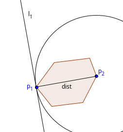
Let $$$p_1$$$ and $$$p_2$$$ be the points that define the diameter of the polygon, e.g. $$$dist(p_1, p_2)$$$ is the maximum possible distance inside the polygon. It is not difficult to see that $$$p_1$$$ and $$$p_2$$$ must lay on the boundary of the polygon, simply because if you draw a line from $$$p_1$$$ to $$$p_2$$$, you're able to extend that line to the boundary, and that way you have found a greater distance. Actually, the two points that define the diameter must be vertices of the polygon. Why? Assume that $$$p_1$$$ lays on an edge of the polygon. Then, there are two directions you could move $$$p_1$$$ to. One of them increases the distance to $$$p_2$$$ and one of them decreases it. Choose the direction that increases the distance and move the point to that direction. This contradicts the assumption that $$$dist(p_1, p_2)$$$ is maximum possible, so the point $$$p_1$$$ cannot lay on the edge of the polygon. We can even prove a stronger result: $$$(p_1, p_2)$$$ is an anti-podal pair!

Construct a circle $$$C$$$ with a center at $$$p_2$$$ and a radius of $$$dist(p_1, p_2)$$$. The points of the polygon must all lay inside the circle, because otherwise $$$p_1$$$ and $$$p_2$$$ wouldn't have the maximum possible distance. Now construct a tangent line $$$l_1$$$ at the point $$$p_1$$$. By definition, the tangent line doesn't intersect the interior of the circle, so it also doesn't intersect the interior of the polygon. Therefore, $$$l_1$$$ has to be a line of support. Now repeat the same procedure with a circle centered around $$$p_1$$$, and the resulting line of support is called $$$l_2$$$. It is easy to see that $$$l_1$$$ and $$$l_2$$$ are parallel to each other. Altogether, the pair $$$(p_1, p_2)$$$ must be an anti-podal pair:

Now that we know that $$$(p_1, p_2)$$$ is an anti-podal pair, we could construct a simple algorithm for calculating the diameter:

1. Calculate all possible anti-podal pairs
2. Return the maximum possible distance of all anti-podal pairs

However, there are two open questions remaining:

1. If we want the algorithm to be efficient, we need to know how many anti-podal pairs there are
2. How can we calculate all possible anti-podal pairs efficiently?

Upper bound on the number anti-podal pairs

Consider any anti-podal pair $$$(p_1, p_2)$$$ (the distance between them doesn't have to be the diameter, it just has to be an anti-podal pair). By definition, there have to be two parallel lines of support $$$l_1, l_2$$$ that intersect the vertices $$$p_1$$$ and $$$p_2$$$ respectively. Now, we can rotate these parallel lines simultaneously until they hit an edge of the polygon. That way, it is possible to map every anti-podal pair to a pair of either two edges or an edge and a vertex. In an algorithm that calculates all anti-podal pairs, it would be sufficient to check for every edge its parallel line of support.

Now there are two cases that need to be considered:

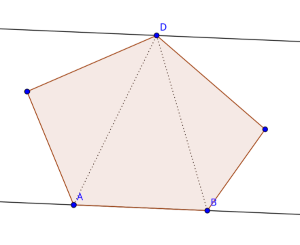
Case 1: The parallel line of support only intersects a vertex. From the image below, we can conclude that there are two anti-podal pairs related to edge $$$AB$$$: The pairs $$$(A, D)$$$ and $$$(B, D)$$$.

Case 2: The parallel line intersects an edge of the polygon. In the image below, we can see that there are 4 possible anti-podal pairs. Since we are looking at two edges however, we can say that each edge accounts for $$$4 / 2 = 2$$$ pairs.

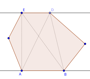
So we can conclude that the number of anti-podal pairs is at most $$$2*n \in O(n)$$$, while $$$n$$$ is the number of edges/vertices of the polygon. Note that it's possible to prove tighter bounds, but for the simplicity of this blog it's enough to have proven that the number of anti-podal pairs is in $$$O(n)$$$.

Algorithm for generating all anti-podal pairs

Our algorithm now consists of iterating over every edge while maintaining a parallel line of support. That's where the rotating calipers technique is going to be used. When going from one edge to the next one, we keep rotating the line of support around the polygon until the lines are parallel again. When an edge is being visited, the anti-podal pairs can be generated the way it was described in the previous section. The algorithm somewhat resembles the two pointer technique. However, as it is with many other geometry problems, the main difficulty does not lay in the description of the solution, but rather in its correct implementation.

In this implementation, the edges are like vectors from one vertex $$$v_i$$$ to the next vertex $$$v_{i+1}$$$. The vertices of the polygon must be sorted in either clockwise or counterclockwise order, the code should work for both. The main difficulty is the criteria on when to stop rotating the parallel line. For that, we'll take a look at an example:

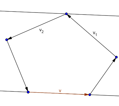
The following two properties hold true:

We observe that there occurs a sign change in the cross product whenever we reach the vertex that allows a parallel line of support. So whenever this occurs, we stop rotating the parallel line. The runtime of this algorithm is $$$O(n)$$$, because iterating over all edges takes $$$O(n)$$$ time, and the parallel line visits every vertex at most once. The implementation:

#define ll long long
#define pii array<int,2>
#define nx(i) (i+1)%n
#define pv(i) (i-1+n)%n

struct Point {
    ll x,y;
 
    Point operator+(const Point &p) {
        return {x + p.x, y + p.y};
    }

    Point operator-(const Point &p) {
        return {x - p.x, y - p.y};
    }
};

ll cross(Point p1, Point p2) {
    return p1.x * p2.y - p1.y * p2.x;
}

int sign(ll num) {
    if (num < 0) return -1;
    else if (num == 0) return 0;
    else return 1;
}

vector<pii> all_anti_podal(int n, vector<Point> &p) {
    int p1 = 0, p2 = 0; // two "pointers"
    vector<pii> result;

    // parallel edges should't be visited twice
    vector<bool> vis(n, false);

    for (;p1<n;p1++) {
        // the edge that we are going to consider in this iteration
        // the datatype is Point, but it acts as a vector
        Point base = p[nx(p1)] - p[p1];

        // the last condition makes sure that the cross products don't have the same sign
        while (p2 == p1 || p2 == nx(p1) || sign(cross(base, p[nx(p2)] - p[p2])) == sign(cross(base, p[p2] - p[pv(p2)]))) {
            p2 = nx(p2);
        }

        if (vis[p1]) continue;
        vis[p1] = true;

        result.push_back({p1, p2});
        result.push_back({nx(p1), p2});
        
        // if both edges from p1 and p2 are parallel to each other
        if (cross(base, p[nx(p2)] - p[p2]) == 0) {
            result.push_back({p1, nx(p2)});
            result.push_back({nx(p1), nx(p2)});
            vis[p2] = true;
        }
    }

    return result;
}

Calculating the width of a convex polygon

Now that we are able to calculate the diameter of a convex polygon, we want to see what other problems we can use the rotating calipers technique for. Let the width of a convex polygon be the shortest distance between two parallel lines of support. The width is like the minimum distance that two walls would need to have such that the entire polygon would fit in between these walls. If the polygon is not convex then we can again just calculate the convex hull and then apply the same procedure.

We can use the same algorithm that we used for the previous problem. We iterate over every edge of the polygon and maintain a parallel line of support $$$l$$$ to the edge. $$$l$$$ can either intersect with an edge or with a vertex of the polygon. Let's look at both of these cases separately:

1. $$$l$$$ intersects with a vertex. Then all you have to do is to calculate the distance from that vertex to the edge.
2. $$$l$$$ intersects with an edge. Select any point on the line $$$l$$$ and calculate the distance to the edge.

After doing all of these calculations, you return the minimum value as the final result. The runtime for this algorithm is $$$O(n)$$$.

Calculating the minimum distance between two convex polygons

Another application for the rotating calipers technique is the problem of the minimum distance between two convex polygons. Note that here, the polygons must be convex from the beginning, unlike in previous problems, where the calculation of a convex hull was sufficient. Additionally we assume that the polygons don't intersect each other, otherwise, the minimum distance would be 0.

Let $$$P$$$ and $$$Q$$$ be two convex polygons, and we want to calculate the minimum distance between them. Let $$$p$$$ and $$$q$$$ be the points that fulfill that minimum distance, e.g. $$$p \in P$$$, $$$q \in Q$$$ and $$$dist(p, q)$$$ is minimum possible. $$$p$$$ and $$$q$$$ must lay on the boundaries of $$$P$$$ and $$$Q$$$ respectively. Furthermore, who would have guessed it, the points $$$p$$$ and $$$q$$$ admit parallel lines of support.

The aforementioned claim is not easy to see, so let's prove it. For that, we need to consider three cases:

Case 1: $$$p$$$ and $$$q$$$ are vertices. We construct a circle $$$C$$$ with $$$q$$$ as a center and $$$dist(p, q)$$$ as the radius. There are obviously no vertices of $$$P$$$ inside $$$C$$$, because that would mean that a smaller distance would be possible. Construct a tangent line $$$l_p$$$ to the circle through $$$p$$$. The claim now is that $$$l_p$$$ is a line of support. Assume that $$$l_p$$$ is not a line of support, e.g. it intersects with the interior of $$$P$$$. Here's an image of what this could look like:

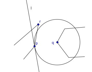
The problem with the assumption becomes pretty clear: A part of the edge between $$$p$$$ and $$$r$$$ lays inside the circle, so a shorter distance than $$$dist(p, q)$$$ is possible. However, that's a contradiction and so $$$l_p$$$ must be a line of support. We can construct another line of support $$$l_q$$$ using the same line of argument. Additionally, $$$l_p$$$ and $$$l_q$$$ are parallel by definition of tangent lines.

Case 2: One point lays on a vertex and the other point on an edge. Without loss of generality, we assume that point $$$p$$$ is a vertex of $$$P$$$ and $$$q$$$ lays on an edge $$$e_q$$$ of $$$Q$$$. Construct a line of support $$$l_p$$$ similar to how it was done in case 1. Now we need to prove that $$$l_p$$$ is parallel to the edge $$$e_q$$$. This follows from the fact that the distance between $$$p$$$ and $$$q$$$ is minimum possible.

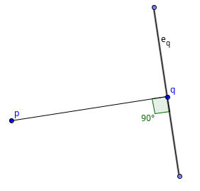
Since the distance between $$$p$$$ and $$$q$$$ is minimum possible, the angle in the image above must be exactly $$$90^{\circ}$$$. The angle between $$$l_p$$$ and the line between $$$p$$$ and $$$q$$$ must be $$$90^{\circ}$$$ as well, therefore, $$$l_p$$$ and the edge $$$e_q$$$ are parallel to each other.

Case 3: Both $$$p$$$ and $$$q$$$ lay on an edge. These edges must be parallel to each other, because if they wouldn't, then we could find a shorter distance where either case 1 or case 2 applies. So, $$$p$$$ and $$$q$$$ also admit parallel lines of support, namely the lines that go through the edges.

The algorithm for minimum distance between two polygons

Now that we know that $$$p$$$ and $$$q$$$ admit parallel lines of support, the rotating calipers algorithm comes back into play. But instead of having two calipers for each polygon, we now have only one caliper per polygon. However, we must pay attention on how we place these calipers initially. If we were to set the calipers like this for example:

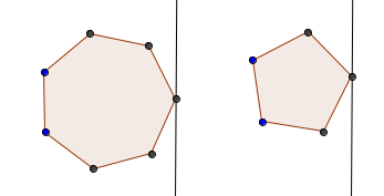
then we could never reach $$$p$$$ and $$$q$$$ at the same time. One way to solve this problem is to initially set the caliper for polygon $$$P$$$ to be a vertical line intersecting with the leftmost vertex of $$$P$$$. Similarly, the caliper for polygon $$$Q$$$ is a vertical line intersecting with the rightmost vertex of $$$Q$$$. As we did for calculating the diameter, we iterate over every edge of $$$P$$$. Let $$$(p_i, p_{i+1})$$$ be the edge of $$$P$$$ that we are currently visiting. Furthermore, let $$$q_j$$$ be the vertex of $$$Q$$$ that is currently visited. We now have to check for all three cases that were mentioned in the last proof:

1. Vertex-vertex case: check $$$dist(p_i, q_j)$$$ and $$$dist(p_{i+1}, q_j)$$$ and update the minimum value accordingly.
2. Edge-vertex case: check the distance between the line segment $$$(p_i, p_{i+1})$$$ and $$$q_j$$$ and update the minimum value accordingly.
3. Edge-edge case: check the distance between the line segments $$$(p_i, p_{i+1})$$$ and $$$(q_j, q_{j+1})$$$. However, this is only possible if these line segments are parallel to each other.

To complete the calculation, you'd have to iterate over all edges of $$$Q$$$ as well. The runtime of this algorithm is $$$O(n+m)$$$, while $$$n = |P|, m = |Q|$$$.

Calculating the maximum distance between two polygons

The algorithm for calculating the minimum distance can be perfectly translated to calculating the maximum distance. The only change one would have to make is to take the maximum over all possible calculated values instead of the minimum. Literally. That's all you have to do. However, if you're fine with an $$$O((n+m)log(n+m))$$$ complexity, I personally would rather recommend calculating the convex hull of the union of both polygons, to then calculate the diameter of the hull.

Conclusion

In this blog, a few basic applications of the rotating calipers technique were discussed. Those are by all means not all applications that exist out there, but rather a few basic ones to understand in which ways we can apply this technique. If you want to submit a solution for the diameter algorithm, you can do it right here. If you have links to additional problems related to this blog, I'd be more than happy to add them to this blog.