Rating changes for last rounds are temporarily rolled back. They will be returned soon. ×

himanshujaju's blog

By himanshujaju, history, 8 years ago, In English

Click here to download the pdf

Pre Requisites

Binary Search — How it works and where can it be applied!

Motivation Problem

We aim to solve this problem : Meteors

The question simply states :

There are N member states and M sectors. Each sector is owned by a member state. There are Q queries, each of which denote the amount of meteor shower in a [L, R] range of sectors on that day. The ith member state wants to collect reqd[i] meteors over all its sectors. For every member state, what is the minimum number of days it would have to wait to collect atleast the required amount of meteors?

Solution

The naive solution here is to do a binary search for each of the N member states. We can update in a range using segment trees with lazy propagation for each query. The time complexity of such a solution would be O(N * logQ * Q * logM). But this one will easily TLE.

Let's see if there's something we are overdoing. For every member state, the binary search applies all the queries until a point multiple times! For example, the first value of mid in the binary search is same for all member states, but we are unnecessarily applying this update everytime, instead of somehow caching it.

Let's do all of these N binary searches in a slightly different fashion. Suppose, in every step we group member states by the range of their binary search. In the first step, all member states lie in range [1, Q]. In the second step, some lie in range [1, Q / 2] while some lie in range [Q / 2, Q] depending on whether the binary search predicate is satisfied. In the third step, the ranges would be [1, Q / 4], [Q / 4, Q / 2], [Q / 2, 3Q / 4], [3Q / 4, Q]. So after logQ steps, every range is a single point, denoting the answer for that member state. Also, for each step running the simulation of all Q queries once is sufficient since it can cater to all the member states. This is pretty effective as we can get our answer in Q * logQ simulations rather than N * Q * logQ simulations. Since each simulation is effectively O(logM), we can now solve this problem in O(Q * logQ * logM).

"A cool way to visualize this is to think of a binary search tree. Suppose we are doing standard binary search, and we reject the right interval — this can be thought of as moving left in the tree. Similarly, if we reject the left interval, we are moving right in the tree.

So what Parallel Binary Search does is move one step down in N binary search trees simultaneously in one "sweep", taking O(N  *  X) time, where X is dependent on the problem and the data structures used in it. Since the height of each tree is LogN, the complexity is O(N  *  X  *  logN)." — animeshf

Implementation

We would need the following data structures in our implementation :

  1. linked list for every member state, denoting the sectors he owns.
  2. arrays L and R denoting range of binary search for each member state.
  3. range update and query structure for Q queries.
  4. linked list check for each mid value of current ranges of binary search. For every mid value, store the member states that need to be checked.

The implementation is actually pretty straight forward once you get the idea. For every step in the simulation, we do the following :

  1. Clear range tree, and update the linked lists for mid values.
  2. Run every query sequentially and check if the linked list for this query is empty or not. If not, check for the member states in the linked list and update their binary search interval accordingly.

Pseudo Code

for all logQ steps:
    clear range tree and linked list check
    for all member states i:
        if L[i] != R[i]:
            mid = (L[i] + R[i]) / 2
            insert i in check[mid]
    for all queries q:
        apply(q)
        for all member states m in check[q]:
            if m has requirements fulfilled:
                R[m] = q
            else:
                L[m] = q + 1

In this code, the apply() function applies the current update, i.e. , it executes the range update on segment tree. Also to check if the requirements are fulfilled, one needs to traverse over all the sectors owner by that member state and find out the sum. In case you still have doubts, go over to the next section and see my code for this problem.

Problems to try

  1. MeteorsMy AC Solution
  2. Make n00b land great again
  3. Travel in HackerLand
  4. SRM 675 Div1 500

Conclusion

I heard about this topic pretty recently, but was unable to find any good tutorial. I picked up this trick from some comments on codeforces blog on Meteors problem. Alternate solutions to the mentioned problems are also welcome, almost every question on parallel binary search can also be solved with some persistent data structure, unless there is a memory constraint. Feel free to point out errors, or make this tutorial better in any way!

Happy Coding!

Full text and comments »

  • Vote: I like it
  • +294
  • Vote: I do not like it

By himanshujaju, history, 9 years ago, In English

You can read the latex formatted pdf here.

Pre Requisites

Dijkstra's algorithm

Motivation Problem

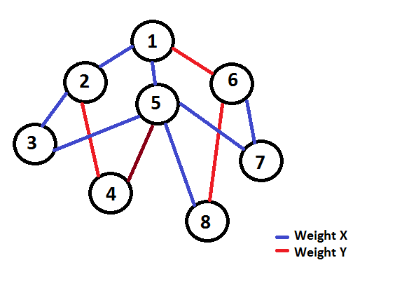
You are given a weighted graph G with V vertices and E edges. Find the shortest path from a given source S to all the vertices, given that all the edges have weight W {X, Y} where X, Y >  = 0

Naive Solution

Most people when given this question would solve it using Dijkstra's algorithm which can solve this efficiently in O(E * logV) (Let's not take Fibonacci heap implementation into consideration now). It turns out that this solution, though it will work in most cases well under the time, can be improved further to a linear time algorithm.

Before moving into the next section, try to think about how you could optimise Dijkstra's algorithm. ( Hint : There are only two possible values of the edge weight.)

Optimised Solution

Let us see why we have the O(logV) factor in the original Dijkstra : priority queue ! So, if we can just find a way to keep the queue sorted by non-decreasing distance in O(1) always, then we can replace the priority queue with a normal queue and find the shortest distance from source to all vertices.

Let us keep two different queues QX and QY. Suppose we are at an arbitrary node u and we are able to reduce the distance to node v by travelling over an edge from u. If this travelled edge from u to v has a weight X then push v to the queue QX, else push it on the queue QY. In short, QX stores information of all nodes whose current minimum is achieved by last travelling over an X weighted edge and QY stores the information of nodes having last weighted edge as Y.

Our entire algorithm is almost the same as that of Dijkstra. One change is to use two queues as mentioned above instead of the priority queue to try and remove the log factor. Another change is that in case of Dijkstra we always take the top node as the next node, but in this algorithm we take the less distant node of the two queue heads. If we can prove that the queues are sorted, we can prove that the answer produced cannot be different from Dijkstra since we are always taking the minimum distant node for calculations and also keeping the distance queues sorted.

Claim : "The queues QX and QY are always sorted."

Proof : Let us assume that the first inversion has just occurred in QX. Let the last element be V and the second last element be U. So, dist(U)  >  dist(V). Now, since both of them last travelled an edge with weight X, we can subtract this quantity from both the distances. Thus, dist(U) - X > dist(V) - X. Let pre(a) = dist(a) - X. Thus, pre(U) > pre(V).

Now, pre(U) and pre(V) must have come from one of the two queues. They cannot come from the same queue, since we assumed the two queues were always sorted before this moment of time. So they must be from two different queues. But according to our algorithm, we take the minimum of the head of the two queues and so if pre(U) was taken before pre(V), then pre(U) <  = pre(V). This contradiction proves that QX is always sorted. We can use a similar argument for the other queue.

Once the claim is proved, the whole algorithm should look pretty trivial from implementation point of view. Since we have removed the log factor, this runs in linear time. We can also extend this to a bigger number of distinct edges and use a set for finding minima. You can refer to the pseudocode in the next section in case you have implementation doubts.

Pseudo Code

queue QX , QY
push source S to QX
while one of the two queues is not empty:
    u = pop minimal distant node among the two queue heads
    for all edges e of form (u,v):
        if dist(v) > dist(u) + cost(e):
            dist(v) = dist(u) + cost(e);
            if cost(e) == X:
                QX.push(dist(v),v);
            else:
                QY.push(dist(v),v);

While finding the minimal distant node, you need to check if anyone of the queue is empty to avoid null pointer errors. Otherwise, everything else is same as Dijkstra when it comes to implementation.

Problems to practice

I don't have any specific problems for this, but all problems that can be solved by 0-1 BFS can also be solved by this. Refer here for some questions.

Conclusion

I hope you learnt something new! Feel free to point out mistakes. There is a rare chance that you would need this algorithm anytime, but it might turn out useful in optimisation problems. This post was largely inspired by a comment on my 0-1 BFS tutorial.

Happy Coding!

Full text and comments »

  • Vote: I like it
  • +92
  • Vote: I do not like it

By himanshujaju, history, 9 years ago, In English

Link to PDF (Latex Formatted)

Topic : Counting Divisors of a Number

Pre Requisites : Basic Maths , Factorisation , Primality testing

Motivation Problem :

There are T test cases. Each test case contains a number N. For each test case , output the number of factors of N.

1 <  = T <  = 10

1 <  = N <  = 1018

Note : 1 and N are also treated as factors of the number N.

Solution :

Naive Solution Factorisation

The most naive solution here is to do the factorisation. But as we can see, it will surely receive the Time Limit Exceeded verdict. You may try to compute the prime numbers till required range and loop over them , but that too exceeds the usual limit of 108 operations. Some optimisations and heuristics may allow you to squeeze through your solution, but usually at the cost of a few TLE's.

Supposing you fit in the above description and cannot think of anything better than the naive solution, I would like to present to you a very simple algorithm which helps you count the number of divisors in , which would be useful for this kind of questions. This algorithm only gives us the count of factors, and not the factors itself.

Firstly, let's do a quick recap of how we obtain the algorithm for any number N :

We write N as product of two numbers P and Q.

Looping over all values of P gives us the count of factors of N.

Before you move forward to the next section, it would be useful if you try to come up with an algorithm that finds the count of factors in . As a hint, the way of thinking is same as that of getting to the algorithm.

Counting factors in

Let's start off with some maths to reduce our factorisation to for counting factors :

We write N as product of three numbers P, Q and R.

We can loop over all prime numbers in range and try to reduce N to it's prime factorisation, which would help us count the number of factors of N.

To know how to calculate divisors using prime factorisation, click here.

We will split our number N into two numbers X and Y such that X * Y = N. Further, X contains only prime factors in range and Y deals with higher prime factors (). Thus, gcd(X , Y) = 1. Let the count of divisors of a number N be denoted by the function F(N). It is easy to prove that this function is multiplicative in nature, i.e., F(m * n) = F(m) * F(n), if gcd(M,N) = 1. So, if we can find F(X) and F(Y), we can also find F(X * Y) or F(N) which is the required quantity.

For finding F(X), we use the naive trial division to prime factorise X and calculate the number of factors. Once this is done, we have Y = N / X remaining to be factorised. This may look tough, but we can see that there are only three cases which will cover all possibilities of Y :

  1. is a prime number : F(Y) = 2.
  2. is square of a prime number : F(Y) = 3.
  3. is product of two distinct prime numbers : F(Y) = 4.

We have only these three cases since there can be at max two prime factors of Y. If it would have had more than two prime factors, one of them would surely have been , and hence it would be included in X and not in Y.

So once we are done with finding F(X) and F(Y), we are also done with finding F(X * Y) or F(N).

Pseudo Code :

N = input()
primes = array containing primes till 10^6
ans = 1
for all p in primes :
            if p*p*p > N:
                  break
            count = 1
            while N divisible by p:
                  N = N/p
                  count = count + 1
            ans = ans * count
if N is prime:
            ans = ans * 2
else if N is square of a prime:
            ans = ans * 3
else if N != 1:
            ans = ans * 4

Checking for primality can be done quickly using Miller Rabin. Thus, the time complexity is for every test case and hence we can solve our problem efficiently.

At this point, you may think that in a similar way, we can reduce this to by handling some cases. I have not thought much on it, but the number of cases to be handled are high since after trial division N could be factorised into one, two or three primes. This is easy enough to code in contest environment, which is our prime objective.

This trick is not quite commonly known and people tend to make bugs in handling the three cases. A problem in regionals which uses this trick directly :

Problem F | Codeforces Gym

You can try also this technique on problems requiring factorisation for practice purposes.

Hope you found this useful! Please suggest more problems to be added as well as any edits, if required.

Happy Coding!

Full text and comments »

  • Vote: I like it
  • +172
  • Vote: I do not like it

By himanshujaju, history, 9 years ago, In English

Link To PDF version (Latex Formatted)

Topic : 0-1 BFS

Pre Requisites : Basics of Graph Theory , BFS , Shortest Path

Problem :

You have a graph G with V vertices and E edges. The graph is a weighted graph but the weights have a contraint that they can only be 0 or 1. Write an efficient code to calculate shortest path from a given source.

Solution :

Naive Solution — Dijkstra's Algorithm.

This has a complexity of O(E + VlogV) in its best implementation. You might try heuristics , but the worst case remains the same. At this point you maybe thinking about how you could optimise Dijkstra or why do I write such an efficient algorithm as the naive solution? Ok , so firstly the efficient solution isn't an optimisation of Dijkstra. Secondly , this is provided as the naive solution because almost everyone would code this up the first time they see such a question , assuming they know Dijkstra's algorithm.

Supposing Dijkstra's algorithm is your best code forward , I would like to present to you a very simple yet elegant trick to solve a question on this type of graph using Breadth First Search (BFS).

Before we dive into the algorithm, a lemma is required to get things crystal clear later on.

Lemma : "During the execution of BFS, the queue holding the vertices only contains elements from at max two successive levels of the BFS tree."

Explanation : The BFS tree is the tree built during the execution of BFS on any graph. This lemma is true since at every point in the execution of BFS , we only traverse to the adjacent vertices of a vertex and thus every vertex in the queue is at max one level away from all other vertices in the queue.

So let's get started with 0-1 BFS.

0-1 BFS :

This is so named , since it works on graphs with edge weights 0 and 1. Let's take a point of execution of BFS when you are at an arbitrary vertex "u" having edges with weight 0 and 1. Similar to Dijkstra , we only put a vertex in the queue if it has been relaxed by a previous vertex (distance is reduced by travelling on this edge) and we also keep the queue sorted by distance from source at every point of time.

Now , when we are at "u" , we know one thing for sure : Travelling an edge (u,v) would make sure that v is either in the same level as u or at the next successive level. This is because the edge weights are 0 and 1. An edge weight of 0 would mean that they lie on the same level , whereas an edge weight of 1 means they lie on the level below. We also know that during BFS our queue holds vertices of two successive levels at max. So, when we are at vertex "u" , our queue contains elements of level L[u] or L[u] + 1. And we also know that for an edge (u,v) , L[v] is either L[u] or L[u] + 1. Thus , if the vertex "v" is relaxed and has the same level , we can push it to the front of our queue and if it has the very next level , we can push it to the end of the queue. This helps us keep the queue sorted by level for the BFS to work properly.

But, using a normal queue data structure , we cannot insert and keep it sorted in O(1). Using priority queue cost us O(logN) to keep it sorted. The problem with the normal queue is the absence of methods which helps us to perform all of these functions :

  1. Remove Top Element (To get vertex for BFS)
  2. Insert At the beginning (To push a vertex with same level)
  3. Insert At the end (To push a vertex on next level)

Fortunately, all of these operations are supported by a double ended queue (or deque in C++ STL). Let's have a look at pseudocode for this trick :

for all v in vertices:
	dist[v] = inf
dist[source] = 0;
deque d
d.push_front(source)
while d.empty() == false:
	vertex = get front element and pop as in BFS.
	for all edges e of form (vertex , u):
		if travelling e relaxes distance to u:
			relax dist[u]
			if e.weight = 1:
				d.push_back(u)
			else:
				d.push_front(u)

As you can see , this is quite similar to BFS + Dijkstra. But the time complexity of this code is O(E + V) , which is linear and more efficient than Dijkstra. The analysis and proof of correctness is also same as that of BFS.

Before moving into solving problems from online judges , try these exercises to make sure you completely understand why and how 0-1 BFS works :

  1. Can we apply the same trick if our edge weights can only be 0 and x (x >= 0) ?
  2. Can we apply the same trick if our edge weights are x and x+1 (x >= 0) ?
  3. Can we apply the same trick if our edge weights are x and y (x,y >= 0) ?

This trick is actually quite a simple trick, but not many people know this. Here are some problems you can try this hack at :

  1. http://www.spoj.com/problems/KATHTHI/My implementation
  2. https://community.topcoder.com/stat?c=problem_statement&pm=10337
  3. Problem J of Gym

Div1 — 500 on topcoder are tough to crack. So congrats on being able to solve one of them using such a simple trick :). I will add more problems as I find.

Happy Coding!

P.S. : My first attempt at a tutorial. Please suggest edits wherever required!

Full text and comments »

  • Vote: I like it
  • +178
  • Vote: I do not like it