lrvideckis's blog

By lrvideckis, history, 6 hours ago, In English

[Tutorial] Schieber & Vishkin LCA Algorithm

The following is a tutorial of the paper: On finding lowest common ancestors: Simplification and parallelization by B Schieber, U Vishkin.

Disclaimer: this technique doesn’t allow one to solve any new problems. Rather it only shaves a log off of some common problems.

To the best of my knowledge, this comment https://mirror.codeforces.com/blog/entry/78931?#comment-655079 was the first time that someone mentioned this algorithm.

Thanks to ssk4988 for giving feedback on this blog.

The Inlabel Numbers

Consider the following code, where adj is the adjacency list of a tree:

int lsb(int x) { return x & -x; } // lsb=least significant bit
int id = 1;
void dfs(int u, int p) {
  for(int v : adj[u]) if(v != p){
    dfs(v, u);
    if(lsb(inlabel[u]) < lsb(inlabel[v])) inlabel[u] = inlabel[v];
  }
  if(!inlabel[u]) inlabel[u] = id++;
}

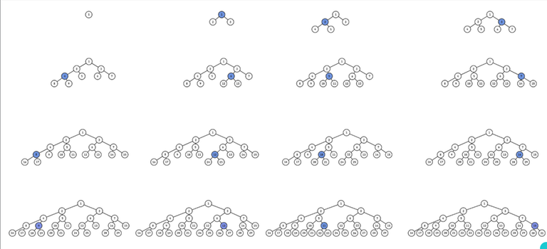
What is this array inlabel? First the leaves have inlabel 1,2,3,... in DFS order.

Photo credits: https://mirror.codeforces.com/blog/entry/132771

Then internal nodes have inlabel equal to the inlabel of one of its children, namely the child whose inlabel has the highest lsb.

To better understand this, observe lsb(8) >= lsb(i) for all i in [1,14]. Thus the 8-th leaf, and all of its ancestors have the same inlabel of 8:

Then 4 and 12 have next highest lsb, thus the 4th and 12th leaf, and all of their ancestors which are not ancestors of the 8th leaf have the same inlabel:

Then 2, 6, 10, 14 have the next highest lsb. We have:

Observe the main 2 facts about the inlabel numbers:

  • They decompose the tree into vertical paths: nodes u and v are on the same vertical path iff inlabel[u]==inlabel[v].
  • You can compress each vertical path into a single node then add edges inlabel[parent[u]] -> inlabel[u]. What you get is not quite a perfect binary tree, rather something similar to a virtual/auxiliary tree of a perfect binary tree. If node u is an ancestor of node v in the original tree, then node inlabel[u] is an ancestor of node inlabel[v] in the perfect binary tree and lsb(inlabel[u]) >= lsb(inlabel[v]).

If nodes u and parent[u] are on different vertical paths, then lsb(inlabel[parent[u]]) > lsb(inlabel[u]). So if you start at u and walk the vertical paths to the root, the lsb’s are strictly increasing, so you’ll walk on at most log(n) paths.

And that’s it! So basically it is a drop-in replacement for HLD.

https://judge.yosupo.jp/submission/367730 https://judge.yosupo.jp/submission/367732

LCA in O(1)

Let LCA(u,v) be a query.

Observe LCA(u,v) is an ancestor of both u and v in the original tree thus inlabel[LCA(u,v)] is an ancestor of both inlabel[u] and inlabel[v] in the perfect binary tree. Thus inlabel[LCA(u,v)] is an ancestor of LCA(inlabel[u], inlabel[v]) in the perfect binary tree.

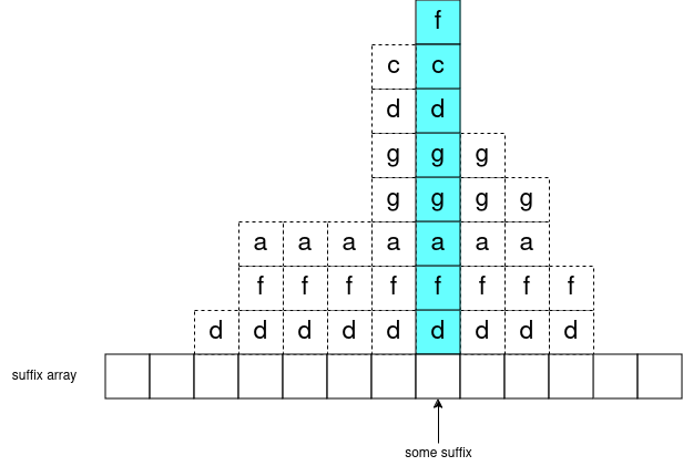
This gives us a starting point. Let’s think about how to calculate LCA(inlabel[u], inlabel[v]). Consider the perfect binary tree and the inlabel’s written vertically in binary:

Observe:

  • The bits more significant than lsb(inlabel[u]) represent the root <-> inlabel[u] path.
  • The bit lsb(inlabel[u]) represents the depth where the root <-> inlabel[u] path stops.

Intuitively, we want to consider the most significant bit where inlabel[u] and inlabel[v] differ as this bit represents the first place where the root <-> inlabel[u] path differs from the root <-> inlabel[v] path. This bit is exactly the bit bit_floor(inlabel[u] ^ inlabel[v]). Formally, we have:

bit_floor(inlabel[u] ^ inlabel[v]) == lsb(LCA(inlabel[u], inlabel[v]))

caveat

It would be so nice if LCA(u,v) always lies on the vertical path corresponding to LCA(inlabel[u], inlabel[v]). But the problem is LCA(u,v) lies on the vertical path corresponding to inlabel[LCA(u,v)] which can be any ancestor of LCA(inlabel[u], inlabel[v]). You could have a case like:

In this case LCA(inlabel[17], inlabel[24]) == 10, but inlabel[LCA(17,24)] == 16. For example, 10 -> 12 -> 8 -> 16 is the path from 10 to 16 in the perfect binary tree.

To fix this problem, we need a new array, ascendant.

The Ascendant Numbers

Definition:

ascendant[root] = lsb(inlabel[root]);
ascendant[u] = ascendant[parent[u]] | lsb(inlabel[u]); // for u != root

Observe if you walk up vertical paths from u to the root, each vertical path corresponds to a bit in ascendant[u]. So you can think of ascendant[u] as storing information about all ancestors of u in some sort of compressed format.

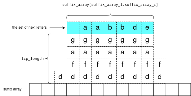
Observe LCA(u,v) is an ancestor of both u and v, thus bit lsb(inlabel[LCA(u,v)]) is set in both ascendant[u] and ascendant[v]. Thus, bit lsb(inlabel[LCA(u,v)]) is set in ascendant[u] & ascendant[v]. In fact, we can say something slightly more general: lsb(inlabel[LCA(u,v)]) is the lowest set bit in ascendant[u] & ascendant[v] which is >= lsb(LCA(inlabel[u], inlabel[v])). Thus, let’s introduce a new variable j:

j = ascendant[u] & ascendant[v] & -bit_floor(inlabel[u] ^ inlabel[v])

First, -bit_floor(inlabel[u] ^ inlabel[v]) can be thought of as a mask that zeros out all lower bits. Next, each bit in j corresponds to some vertical path containing or above LCA(u,v). For example, we have: lsb(j) == lsb(inlabel[LCA(u,v)]).

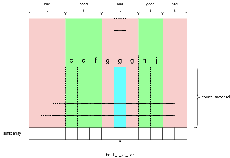
Then if we do: ascendant[u] ^ j (ascendant[u] - j also works), we xor-ed out all the high bits in ascendant[u]. What we’re left with are the lower bits corresponding to the vertical paths strictly below LCA(u,v).

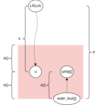
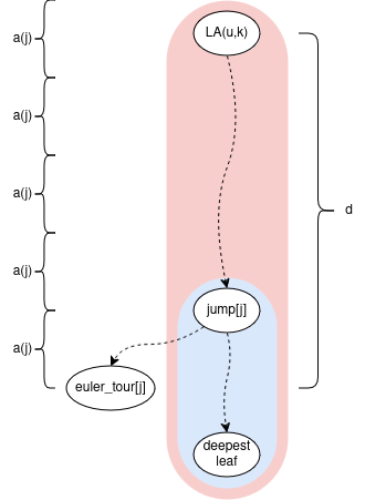
Let’s introduce a new variable k as k=bit_floor(ascendant[u] ^ j), representing the highest vertical path strictly below LCA(u,v). One final property of inlabel numbers is (inlabel[u] & -k) | k is the ancestor of inlabel[u] in the perfect binary tree such that lsb(inlabel[u] & -k) | k) == k.

If we precalculate an array head which maps inlabel numbers to the head (node closest to root) of the corresponding vertical path, then parent[head[(inlabel[u] & -k) | k]] represents the lowest ancestor of u on the same vertical path as LCA(u,v). We do the same for v, then LCA(u,v) is the node closer to the root.

We only jump up u if it’s not on the same vertical path as LCA(u,v), i.e. if inlabel[u] != inlabel[LCA(u,v)]. (And similarly for v). For example if inlabel[u]==inlabel[v] initially, then we don't jump up either node and LCA(u,v) is just the node closer to the root.

https://judge.yosupo.jp/submission/367724

<O(n),O(1)> Almost-LCA in Tree

Problem: https://mirror.codeforces.com/blog/entry/71567

Assume we have u,v, where u != v.

If ascendant[u] is not a submask of ascendant[v], then u is not an ancestor of v. The answer is parent[u].

Else, ascendant[u] is a submask of ascendant[v]. Then each bit in ascendant[u] ^ ascendant[v] corresponds to a vertical path below LCA(u,v). Let’s find the highest set bit with:

k = bit_floor(ascendant[u] ^ ascendant[v])

Then jump up v with: v = head[(inlabel[v] & -k) | k]. Now it’s just a few cases:
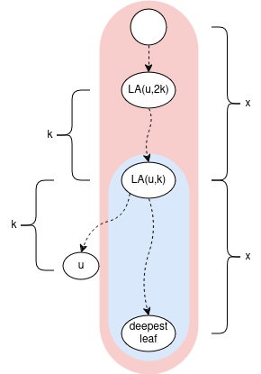
  • If parent[v] == u then answer is v
  • Else if depth[u] < depth[v] then the next node on path is the child of u with the same inlabel as u (precompute this in an array)
  • Else u is not an ancestor of v. The answer is parent[u].

Open Problem

I thought a lot but couldn’t solve it myself. Also I was unable to get AI to solve it. I’d love to know an answer to it.

Currently, it requires 2 DFS’s. In the first DFS, the inlabel numbers are calculated bottom-up. Then in the second DFS, the ascendant numbers are calculated top-town and depend on the inlabel numbers.

The open problem is can you do it in a single DFS. Maybe there’s some alternative to the ascendant numbers which can be calculated in the first DFS alongside with the inlabel numbers which also allows O(1) LCA.

If you use this as a replacement for HLD, then you need 2 DFS’s anyways, but if you use this only for LCA, then a single DFS solution would be nice to have.

Full text and comments »

  • Vote: I like it
  • +13
  • Vote: I do not like it

By lrvideckis, history, 14 months ago, In English

For the longest time, this comment https://mirror.codeforces.com/blog/entry/112755#comment-1004966 was bugging me (the part about how the 'complete' segment tree is 20% slower (complete, because it’s a complete binary tree)). Instead of benchmarking, this blog calculates the expected number of recursive calls visited between segment tree implementations.

Thanks to camc for giving valuable feedback.

This blog will study 2 implementations of segment trees.

'standard' segment tree

And

'complete' segment tree

(complete, because it’s a complete binary tree); Also tourist uses the iterative version of this.

Structure

Consider the structures of 'standard' segment trees on n=1,2,3,...

(credit to this tool for making the pictures; here are the pictures in higher resolution)

Notice going from one tree to the next, exactly one leaf node turns into an internal node, and “grows” 2 new leaves. Well consider the sequence of the nodes which “grow” 2 new leaves:

1, 2, 3, 4, 6, 5, 7, 8, 12, 10, 14, 9, 13, 11, 15, …

It is exactly this sequence https://oeis.org/A059893. But this sequence is about reversing bits, so how is it related?

As you increment n, the child (left or right) of the root whose range-size increments will alternate (so it’s based on parity/LSB of n), then the child’s range-size is half of the root’s range-size and you repeat to determine which grandchild’s range-size increments (it also alternates), and so on. Eventually you get to a leaf, and this leaf’s range-size increments (i.e. “grows” 2 new leaves).

If you split up the sequence into subarrays [1,2), [2,4), [4,8), ..., [2^(i-1),2^i),..., then:

  • the i-th subarray represents all nodes at depth i
  • Every node at depth i grows its leaves before all nodes at depth (i+1), and after all nodes at depth (i-1)
  • So as n increases, the standard segment tree grows its leaves layer by layer, i.e. each layer is completed fully before the next layer’s leaves start growing.
  • abs(depth(leaf_i)-depth(leaf_j))<=1 for any pairs of leaves

Point updates/queries

Expected number of recursive calls of point update

= expected depth of leaf node (where depth of root=1)

= sum_of_leaf_depths/n

So how to work out the sum of depths of leaves?

Well there are x leaves of depth __lg(n)+1 and y leaves of depth __lg(n)+2. We have:

  • x+y=n
  • y = 2*(bit_floor(n)-x) because there are bit_floor(n)-x internal nodes at depth __lg(n)+1, each having 2 leaf-childs.

Then sum of depths of leaves = x*(__lg(n)+1)+y*(__lg(n)+2).

Finally notice, this math is exactly the same for both the complete segment tree and the standard segment tree, so they have the same sum of leaf depths.

Also for merge sort tree: (sum of array lengths) = (sum of leaf depths). So the respective merge sort tree’s have the same sum of array lengths.

Range updates/queries

Expected number of recursive calls of range update

= total_recursive_calls_over_all_possible_updates/(n*(n+1)/2)

Test comparing total number of recursive calls

I was blown away by this. I thought that the complete segment tree should have more recursive calls because the ranges aren’t split in the middle. But somehow this is wrong? Let’s see why.

I was able to come up with this formula for the total number of recursive calls (derivation left to the reader haha).

formula

Comparing this formula for complete versus standard segment tree:

  • (-7n^2-3n+4)/2 is the same
  • sum of [depth*(2n+3)] over leaves is the same as they both have the same number of leaves at depths __lg(n)+1 and __lg(n)+2

The only difference is we subtract f(n) = n^2 + f(left child range-size) + f(right child range-size) from the total number of calls. And f(n) increases when abs(left child range-size - right child range-size) increases, i.e. as the tree becomes less balanced.

To me, this result is unintuitive. I’d be interested if anyone can come up with some intuition for this.

But then why is the complete segment tree slower...

Calculating the midpoint has a larger constant.

Full text and comments »

  • Vote: I like it
  • +52
  • Vote: I do not like it

By lrvideckis, history, 20 months ago, In English

Recently I was learning about how to binary search over suffix array to solve string matching (specifically, single text, multiple patterns, solve it online). Here (1 ("Pattern Query" section), 2, 3) describes how to solve it in O(|s| * log(|p|)) but I'll describe how to improve this to O(|s| + log(|p|)). There already exists resources online about this, but I will try to simplify it.

visualizing suffix array

Let's take the text s="banana", and consider all suffixes (written vertically):

a
n a
a n a
n a n a
a n a n a
b a n a n a
0 1 2 3 4 5

now let's sort it:

      a
    a n
    n a   a
  a a n   n
  n n a a a
a a a b n n
5 3 1 0 4 2

s's suffix array is [5, 3, 1, 0, 4, 2].

Now take any substring of s (like "an"). Observe there exists a maximal-length subarray of s's suffix array ([3,1]) representing all the suffixes (3 -> "ana", 1 -> "anana") where "an" is a prefix. I like to call this the "subarray of matches": as this subarray represents all the starting indexes (in s) of a match.

Let's define a function which calculates this: subarray_of_matches(s[s_l:s_r]) = suffix_array[suffix_array_l:suffix_array_r].

Now observe that subarray_of_matches(s[s_l:s_r+1]) is nested inside subarray_of_matches(s[s_l:s_r]). This is because every spot where s[s_l:s_r+1] is a match, s[s_l:s_r] is also a match.

But in particular, we can take some suffix (like "anana") and plug in all of its' prefixes to subarray_of_matches and we get a sequence of nested subarrays:

subarray_of_matches("a") = [5,3,1]
subarray_of_matches("an") = [3,1]
subarray_of_matches("ana") = [3,1]
subarray_of_matches("anan") = [1]
subarray_of_matches("anana") = [1]

in general, you can visualize it like this:

One more point: consider any subarray of the suffix array: suffix_array[suffix_array_l:suffix_array_r] and let lcp_length = the longest common prefix of these suffixes. Formally: for each i in range [suffix_array_l,suffix_array_r) the strings s[suffix_array[i]:suffix_array[i]+lcp_length] are all equal.

Now consider the set of next letters: s[suffix_array[i]+lcp_length], they are sorted. We can visualize it like:

visualizing the binary search

Given text s, s's suffix array, and query string p, our goal is to calculate the minimum index i such that p is a prefix of s[suffix_array[i]:] (the suffix of s starting at suffix_array[i])

so we can start the binary search as usual with l=0,r=size(s),m=(l+r)/2, and compare p to s[suffix_array[m]:]. if p is less, search lower (r=m;), else search higher (l=m;).

Let's also keep track of the "best" suffix so far, e.g. the suffix which matches the most characters in p. Let's store it as a pair {best_i_so_far,count_matched} with the invariant: p[:count_matched] == s[best_i_so_far:best_i_so_far+count_matched].

So now, depending on whether p[:count_matched+1] is less/greater than s[best_i_so_far:best_i_so_far+count_matched+1] we want to look for the green section which is before/after best_i_so_far. And here, we have the cases taken from here:

  • the middle red section will not contain the answer because the pattern p didn't match with that letter g, so it still won't match anywhere in that range.

  • the green sections will contain a match which is either better or the same as the middle red section

  • the outer red sections won't contain the answer because the LCP is too low

So back to our binary search, we have l,r,m=(l+r)/2.

  • If m lies in either of the red sections; then we can check for this in O(1) using a lcp query, and continue the search "towards" the green section.

  • If m is already in the green section, then continue matching p[count_matched:] with s[best_i_so_far+count_matched:] (and also update our best match {best_i_so_far,count_matched})

we start comparing characters in p starting from count_matched, so we only compare characters in p once, and achieve complexity O(log(|s|) + |p|).

code: https://mirror.codeforces.com/edu/course/2/lesson/2/3/practice/contest/269118/submission/277693465

Full text and comments »

  • Vote: I like it
  • +47
  • Vote: I do not like it

By lrvideckis, history, 2 years ago, In English

I recently read “Still Simpler Static Level Ancestors by Torben Hagerup” describing how to process a rooted tree in O(n) time/space to be able to answer online level ancestor queries in O(1). I would like to explain it here. Thank you to camc for proof-reading & giving feedback.

background/warmup

Prerequisites: ladder decomposition: https://mirror.codeforces.com/blog/entry/71567?#comment-559299, and <O(n),O(1)> offline level ancestor https://mirror.codeforces.com/blog/entry/52062?#comment-360824

First, to define a level ancestor query: For a node u, and integer k, let LA(u, k) = the node k edges “up” from u. Formally a node v such that:

  • v is an ancestor of u
  • distance(u, v) = k (distance here is number of edges)

For example LA(u, 0) = u; LA(u, 1) = u’s parent

Now the slowest part of ladder decomposition is the O(n log n) binary lifting. Everything else is O(n). So the approach will be to swap out the binary lifting part for something else which is O(n).

We can do the following, and it will still be O(n):

  • Store the answers to O(n) level ancestor queries of our choosing (answered offline during the initial build)
  • Normally in ladder decomposition, length(ladder) = 2 * length(vertical path). But we can change this to length(ladder) = c * length(vertical path) for any constant c (of course the smaller the better).

The key observation about ladders: Given any node u and integer k (0 <= k <= depth[u] / 2): The ladder which contains LA(u, k) also contains LA(u, 2*k); or generally LA(u, c*k) when we extend the vertical paths by the multiple of c.

the magic sequence

Let’s take a detour to the following sequence a(i) = (i & -i) = 1 << __builtin_ctz(i) for i >= 1 https://oeis.org/A006519

1 2 1 4 1 2 1 8 1 2 1 4 1 2 1 16 1 2 1 4 1 2 1 8 1 2 1 4 1 2 1 32 1 2 1 4 1 2 1 …

Observe: for every value 2^k, it shows up first at index 2^k (1-based), then every 2^(k+1)-th index afterwards.

Q: Given index i >=1, and some value 2^k, I can move left or right. What’s the minimum steps I need to travel to get to the nearest value of 2^k?

A: at most 2^k steps. The worst case is I start at a(i) = 2^l > 2^k, e.g. exactly in the middle of the previous, and next occurrence of 2^k

the algorithm

Let’s do a 2n-1 euler tour; let the i’th node be euler_tour[i]; i >= 1. Let’s calculate an array jump[i] = LA(euler_tour[i], a(i)) offline, upfront.

how to use the “jump” array to handle queries?

Let node u, and integer k be a query. We can know i = u’s index in the euler tour (it can show up multiple times; any index will work).


key idea: We want to move either left, right in the euler tour to find some “close”-ish index j with a “big” jump upwards. But not too big: we want to stay in the subtree of LA(u,k). Then we use the ladder containing jump[j] to get to LA(u,k). The rest of the blog will be the all math behind this.


It turns out we want to find closest index j such that 2*a(j) <= k < 4*a(j). Intuition: we move roughly k/2 steps away in the euler tour to get to a node with an upwards jump of size roughly k/2.

Note if we move to j: abs(depth[euler_tour[i]] - depth[euler_tour[j]]) <= abs(i - j) <= a(j)

how to calculate j in O(1)

Note we’re not creating a ladder of length c*a(i) starting from every node because that sums to c*(a(1)+a(2)+...+a(2n-1)) = O(nlogn). Rather it’s a vertical path decomposition (sum of lengths is exactly n), and each vertical path is extended upwards to c*x its original length into a ladder (sum of lengths <= c*n)

finding smallest c for ladders to be long enough

Let’s prove some bounds on d = depth[euler_tour[j]] - depth[LA(u,k)]

Note 2*a(j) <= k from earlier. So a(j) = 2*a(j) - a(j) <= k - a(j) <= d. This implies jump[j] stays in the subtree of LA(u,k).

Note k < 4*a(j) from earlier. So d <= a(j) + k < a(j) + 4*a(j) = 5*a(j)

Remember, we can choose a constant c such that length(ladder) = c * length(vertical path). Now let’s figure out the smallest c such that the ladder containing jump[j] will also contain LA(u,k):

if we choose c=5 then length(ladder) = 5 * length(vertical path) >= 5 * a(j) > d

I mean that constant factor kinda sucks :( Well, at least we’ve shown a way to do the almighty, all-powerful theoretical O(n)O(1) level ancestor, all hail to the almighty. If thou is tempted by method of 4 russians, thou shall receive eternal punishment

here’s a submission with everything discussed so far: https://judge.yosupo.jp/submission/194335

a cool thing

Here’s some intuition for why we chose the sequence a(i): It contains arbitrarily large jumps which appear regularly, sparsely. Sound familiar to any algorithm you know? It feels like linear jump pointers https://mirror.codeforces.com/blog/entry/74847. Let’s look at the jump sizes for each depth:

1,1,3,1,1,3,7,1,1,3,1,1,3,7,15,1,1,3,...

Map x -> (x+1)/2 and you get https://oeis.org/A182105 . https://oeis.org/A006519 is kinda like the in-order traversal of a complete binary tree, and https://oeis.org/A182105 is like the post-order traversal.

improving the constant factor

Let’s introduce a constant kappa (kappa >= 2).

Instead of calculating jump[i] as LA(euler_tour[i], a(i)), calculate it as LA(euler_tour[i], (kappa-1) * a(i))

Let node u, and integer k be a query. We want to find nearest j such that kappa*a(j) <= k < 2*kappa*a(j)

Then you can bound d like: (kappa-1) * a(j) <= d < (2 * kappa + 1) * a(j)

And you can show c >= (2 * kappa + 1) / (kappa - 1)

The catch is when k < kappa, you need to calculate LA(u,k) naively (or maybe store them).

The initial explanation is for kappa = 2 btw

submission with kappa: https://judge.yosupo.jp/submission/194336

Full text and comments »

  • Vote: I like it
  • +125
  • Vote: I do not like it

By lrvideckis, history, 2 years ago, In English

I came across this paper

On Finding Lowest Common Ancestors: Simplification and Parallelization by Baruch Schieber, Uzi Vishkin April, 1987

so naturally I tried to code golf it

lca https://judge.yosupo.jp/submission/360243

rmq https://judge.yosupo.jp/submission/360244

Full text and comments »

  • Vote: I like it
  • +90
  • Vote: I do not like it

By lrvideckis, history, 3 years ago, In English

Hi Codeforces! If you calculate midpoint like

int get_midpoint(int l, int r) {//[l, r)
	int pow_2 = 1 << __lg(r-l);//bit_floor(unsigned(r-l));
	return min(l + pow_2, r - pow_2/2);
}

then your segment tree requires only $$$2 \times n$$$ memory.

test
proof

I was inspired by ecnerwala's in_order_layout https://github.com/ecnerwala/cp-book/blob/master/src/seg_tree.hpp

I'll be waiting for some comment "It's well known in china since 2007" 😂

Full text and comments »

  • Vote: I like it
  • +64
  • Vote: I do not like it

By lrvideckis, history, 6 years ago, In English

Here are some reasons I believe people do CP:

  • Enjoyment
  • Preparation for job (coding) interviews
  • Preparation for Competitions

CP seems to be a low priority activity. For example, school and job responsibilities usually take higher priority. It’s not possible (realistically) to make a living from CP. Thus, people taking part in CP usually have good reasons.

The nihilist viewpoint says CP is just solving contrived made-up problems. Who cares? There’s little/no benefit to society. Unlike CP, programming for a job creates services (value) for people. Unlike CP, Computer Science research pushes the boundaries of knowledge of the field (value). Why spend time in an activity which doesn’t product relative value? Again, it seems the people doing CP must have good reasons.

I’m wondering what people’s reasons are for doing CP.

Full text and comments »

  • Vote: I like it
  • +129
  • Vote: I do not like it