Hi all,

I would like to share with you a part of my undergraduate thesis on a Multi-String Pattern Matcher data structure. In my opinion, it's easy to understand and hard to implement correctly and efficiently. It's competitive against other MSPM data structures (Aho-Corasick, suffix array/automaton/tree to name a few) when the dictionary size is specifically (uncommonly) large.

I would also like to sign up this entry to bashkort's Month of Blog Posts:-)

Abstract

This work describes a hash-based mass-searching algorithm, finding (count, location of first match) entries from a dictionary against a string $$$s$$$ of length $$$n$$$. The presented implementation makes use of all substrings of $$$s$$$ whose lengths are powers of $$$2$$$ to construct an offline algorithm that can, in some cases, reach a complexity of $$$O(n \log^2n)$$$ even if there are $$$O(n^2)$$$ possible matches. If there is a limit on the dictionary size $$$m$$$, then the precomputation complexity is $$$O(m + n \log^2n)$$$, and the search complexity is bounded by $$$O(n\log^2n + m\log n)$$$, even if it performs in practice like $$$O(n\log^2n + \sqrt{nm}\log n)$$$. Other applications, such as finding the number of distinct substrings of $$$s$$$ for each length between $$$1$$$ and $$$n$$$, can be done with the same algorithm in $$$O(n\log^2n)$$$.

Problem Description

We want to write an offline algorithm for the following problem, which receives as input a string $$$s$$$ of length $$$n$$$, and a dictionary $$$ts = \{t_1, t_2, .., t_{\lvert ts \rvert}\}$$$. As output, it expects for each string $$$t$$$ in the dictionary the number of times it is found in $$$s$$$. We could also ask for the position of the fist occurrence of each $$$t$$$ in $$$s$$$, but the paper mainly focuses on the number of matches.

Algorithm Description

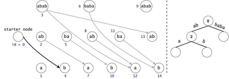
We will build a DAG in which every node is mapped to a substring from $$$s$$$ whose length is a power of $$$2$$$. We will draw edges between any two nodes whose substrings are consecutive in $$$s$$$. The DAG has $$$O(n \log n)$$$ nodes and $$$O(n \log^2 n)$$$ edges.

We will break every $$$t_i \in ts$$$ down into a chain of substrings of $$$2$$$-exponential length in strictly decreasing order (e.g. if $$$\lvert t \rvert = 11$$$, we will break it into $$$\{t[1..8], t[9..10], t[11]\}$$$). If $$$t_i$$$ occurs $$$k$$$ times in $$$s$$$, we will find $$$t_i$$$'s chain $$$k$$$ times in the DAG.

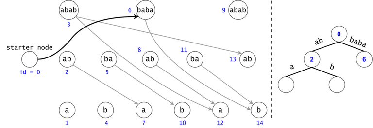
Figure 1: The DAG for $$$s = (ab)^3$$$. If $$$ts = \{aba, baba, abb\}$$$, then $$$t_0 = aba$$$ is found twice in the DAG, $$$t_1 = baba$$$ once, and $$$t_2 = abb$$$ zero times.

Redundancy Elimination: Associated Trie, Tokens, Trie Search

A generic search for $$$t_0 = aba$$$ in the DAG would check if any node marked as $$$ab$$$ would have a child labeled as $$$a$$$. $$$t_2 = abb$$$ is never found, but a part of its chain is ($$$ab$$$). We have to check all $$$ab$$$s to see if any may continue with a $$$b$$$, but we have already checked if any $$$ab$$$s continue with an $$$a$$$ for $$$t_0$$$, making second set of checks redundant.

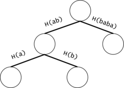
Figure 2: If the chains of $$$t_i$$$ and $$$t_j$$$ have a common prefix, it is inefficient to count the number of occurrences of the prefix twice. We will put all the $$$t_i$$$ chains in a trie. We will keep the hashes of the values on the trie edges.

In order to generalize all of chain searches in the DAG, we will add a starter node that points to all other nodes in the DAG. Now all DAG chains begin in the same node.

The actual search will go through the trie and find help in the DAG. The two Data Structures cooperate through tokens. A token is defined by both its value (the DAG index in which it’s at), and its position (the trie node in which it’s at).

Trie Search steps

The single token present at the start of the search is the Starter Node's token, located in the trie's root. We try to propagate it by seeing if any edges ongoing from the Starter Node end in a node labeled on the trie edges (children of the trie node containing the token).

Particularly, we try to see if $$$a \in \{ab, baba\}$$$ (in practice, we compare hashes). Since the membership test failed, we can't propagate the $$$0$$$ token on this DAG edge.

We move on to the next edge coming out of the Starter node. $$$ab \in \{ab, baba\}$$$, so the $$$0$$$ token produces a child, the $$$2$$$ token. We are trying to "tape together" as much from the DAG as we can to the trie.

$$$abab \notin \{ab, baba\}$$$.

$$$b \notin \{ab, baba\}$$$.

We skip a number of Starter Node children until we get the next one that propagates.

We skip again.

This is the last Starter Node child that propagated.

We now try to propagate the newly formed tokens. The token marked as $$$2$$$ only has one outgoing edge in the DAG. $$$a \in \{a, b\}$$$, so we get a new token, $$$7$$$.

$$$8$$$ also propagates, spawning $$$12$$$. $$$13$$$ doesn't have any DAG children, so it can't propagate, ending the Trie Search. We have found the strings $$$ab$$$ three times, $$$aba$$$ twice, and $$$baba$$$ once.

Token count bound and Token propagation complexity

Property 1: There is a one-to-one mapping between tokens and $$$s$$$’ substrings. Any search will generate $$$O(n^2)$$$ tokens.

Proof 1: If two tokens would describe the same substring of $$$s$$$ (value-wise, not necessarily position-wise), they would both be found in the same trie node, since the described substrings result from the concatenation of the labels on the trie paths from the root.

Now, since the two tokens are in the same trie node, they can either have different DAG nodes attached (so different ids), meaning they map to different substrings (i.e. different starting positions), or they belong to the same DAG node, so one of them is a duplicate: contradiction, since they were both propagated from the same father.

As a result, we can only generate in a search as many tokens as there are substrings in $$$s$$$, $$$n(n+1)/2 + 1$$$, also accounting for the empty substring (Starter Node's token). $$$\square$$$

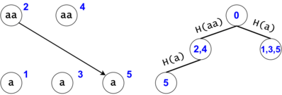
Figure 3: $$$s = aaa, ts = \{a, aa, aaa\}$$$. There are two tokens that map to the same DAG node with the id $$$5$$$, but they are in different trie nodes: one implies the substring $$$aaa$$$, while the other implies (the third) $$$a$$$.

Property 2: Ignoring the Starter Node's token, any token may divide into $$$O(\log n)$$$ children tokens. We can propagate a child in $$$O(1)$$$ (the cost of the membership test (in practice, against a hashtable containing rolling hashes passed through a Pseudo-Random Function)).

As a result, we have a pessimistic bound of $$$O(n^2 \log n)$$$ for a search.

Another redundancy: DAG suffix compression

Property 3: If we have two different tokens in the same trie node, but their associated DAG nodes’ subtrees are identical, it is useless to propagate the second token anymore. We should only propagate the first one, and count twice any finding that it will have.

Proof 3: If we don’t merge the tokens that respect the condition, their children will always coexist in any subsequent trie nodes: if one gets propagated, the other will as well, or none get propagated. We can apply this recursively to cover the entire DAG subtree. $$$\square$$$

Intuitively, we can consider two tokens to be the same if their future cannot be different, no matter their past.

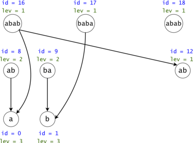
Figure 4: The DAG from Figure 1 post suffix compression. We introduce the notion of leverage. If we compress $$$k$$$ nodes into each other, the resulting one will have a leverage equal to $$$k$$$. We were able to compress two out of the three $$$ab$$$ nodes. If we are to search now for $$$aba$$$, we would only have to only propagate one token $$$ab \rightarrow a$$$ instead of the original two.

Property 4: The number of findings given by a compressed chain is the minimum leverage on that chain (i.e. we found $$$bab$$$ $$$\min([2, 3]) = 2$$$ times, or $$$ab$$$ $$$\min([2]) + \min([1]) = 3$$$ times). Also, the minimum on the chain is always given by the first DAG node on the chain (that isn't the Starter Node).

Proof 4: Let $$$ch$$$ be a compressed DAG chain. If $$$1 \leq i < j \leq \lvert ch \rvert$$$, then $$$node_j$$$ is in $$$node_i$$$'s subtree. The more we go into the chain, the less restrictive the compression requirement becomes (i.e. fewer characters need to match to unite two nodes).

If we united $$$node_i$$$ with another node $$$x$$$, then there must be a node $$$y$$$ in $$$x$$$'s subtree that we can unite with $$$node_j$$$. Therefore, $$$lev_{node_i} \leq lev_{node_j}$$$, so the minimum leverage is $$$lev_{node_1}$$$. $$$\square$$$