Introduction
This is a tutorial/exploration of problems that can be solved using the "DFS tree" of a graph.
For a way too long time, I didn't really understand how and why the classical algorithm for finding bridges works. It felt like many tutorials didn't really explain how it works, kind of just mentioned it in passing and quickly just moved on to implementation. The day someone explained what the DFS tree is, I finally understood it properly. Before, it took me ages to implement bridge-finding properly, and I always had to look up some detail. Now I can implement it at typing speed.
But more importantly, I began to see how the same techniques can be used to solve graph problems that have more or less nothing to do with bridges. The thing is, when you have a black box, you can only ever use it as a black box. But if you have a box that you understand well, you can take it into pieces, repurpose the pieces for completely different things, all without getting lost.
In my opinion, the DFS tree one of the most useful techniques for solving structural problems about graphs that I know of. Also, sometimes there are questionable greedy algorithms whose correctness becomes obvious once you think about the DFS tree.
The DFS tree
Consider an undirected connected graph $$$G$$$. Let's run a depth-first traversal of the graph. It can be implemented by a recursive function, perhaps something like this:
1 function visit(u):
2     mark u as visited
3     for each vertex v among the neighbours of u:
4         if v is not visited:
5             mark the edge uv
6             call visit(v)
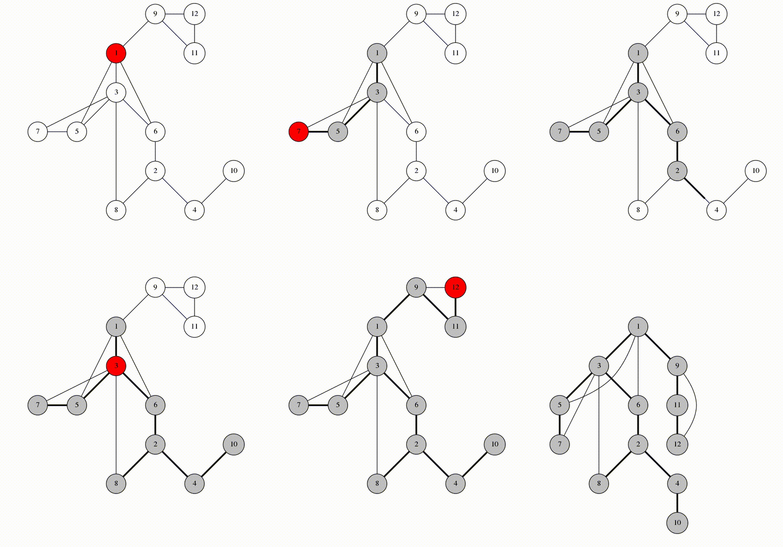
Here is an animation of what calling visit(1) looks like.

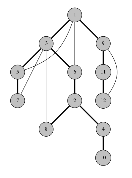
Let's look at the edges that were marked in line 5. They form a spanning tree of $$$G$$$, rooted at the vertex 1. We'll call these edges span-edges; all other edges are called back-edges.
This is the DFS tree of our graph:

Observation 1. The back-edges of the graph all connect a vertex with its descendant in the spanning tree. This is why DFS tree is so useful.
For example in the graph above, vertices 4 and 8 couldn't possibly have a back-edge connecting them because neither of them is an ancestor of the other. If there was an edge between 4 and 8, the traversal would have gone to 8 from 4 instead of going back to 2.
This is the most important observation about about the DFS tree. The DFS tree is so useful because it simplifies the structure of a graph. Instead of having to worry about all kinds of edges, we only need to care about a tree and some additional ancestor-descendant edges. This structure is so much easier to think and write algorithms about.
Finding bridges (or articulation points)
The DFS tree and observation 1 are the core of Tarjan's bridge-finding algorithm. Typical tutorials about finding bridges only mention the DFS tree in passing and start by defining weird arrays like $$$\mathrm{dfs}[u]$$$ and $$$\mathrm{low}[u]$$$: forget all that. These are implementation details, and in my opinion this isn't even the most intuitive way to implement finding bridges. In bridge-finding, $$$\mathrm{dfs}[u]$$$ is simply an obfuscated way to check whether one vertex is an ancestor of another in the DFS tree. Meanwhile it is even kind of hard to clearly explain what $$$\mathrm{low}[u]$$$ is supposed to represent.
Here's how to find bridges in an undirected connected graph $$$G$$$. Consider the DFS tree of $$$G$$$.
Observation 2. A span-edge $$$uv$$$ is a bridge if and only if there exists no back-edge that connects a descendant of $$$uv$$$ with an ancestor of $$$uv$$$. In other words, a span-edge $$$uv$$$ is a bridge if and only if there is no back-edge that "passes over" $$$uv$$$.
For example, in the DFS tree above, the edge between 6 and 2 isn't a bridge, because even if we remove it, the back-edge between 3 and 8 holds the graph together. On the other hand, the edge between 2 and 4 is a bridge, because there is no back-edge passing over it to hold the graph together if $$$2-4$$$ is removed.
Observation 3. A back-edge is never a bridge.
This gives rise to the classical bridge-finding algorithm. Given a graph $$$G$$$:
- find the DFS tree of the graph;
- for each span-edge $$$uv$$$, find out if there is a back-edge "passing over" $$$uv$$$, if there isn't, you have a bridge.
Because of the simple structure of the DFS tree, step 2 is easy to do. For example, you can use the typical $$$\mathrm{low}[u]$$$ method. Or, for example, you can use some kind of prefix sums, which is what I prefer. I define $$$\mathrm{dp}[u]$$$ as the number of back-edges passing over the edge between $$$u$$$ and its parent. Then,
The edge between $$$u$$$ and its parent is a bridge if and only if $$$\mathrm{dp}[u] = 0$$$.
Directing edges to form a strongly connected graph
Consider the following problem. Unfortunately I don't know if you can submit solutions somewhere. This is 118E - Bertown roads.
Problem 1. You are given an undirected connected graph $$$G$$$. Direct all of its edges so that the resulting digraph is strongly connected, or declare that this is impossible.
I know of a solution without using the ideas of DFS tree in linear time, but it is quite annoying and I would never want to implement this. Meanwhile, a DFS tree solution is very easy to implement in only a few lines of code.
Observation 4. If $$$G$$$ contains bridges, this is impossible.
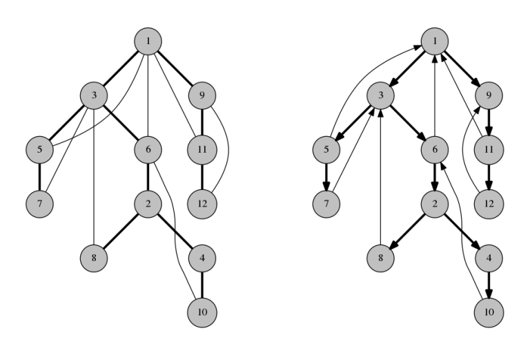
So from now on, suppose that the graph doesn't have bridges. Let's look at its DFS tree. Direct all span-edges downwards and all back-edges upwards.

Observation 5. There is a path from the root to each vertex.
Observation 6. There is a path from each vertex to the root.
Therefore, the graph is now strongly connected! This solution can be implemented without an explicit reference to the DFS tree, but it is a very good example of proving the correctness using DFS tree.
Implementing cacti
Sometimes the DFS tree is just a way to represent a graph that makes implementation of certain things convenient. Like an adjacency list but "next level". This section is purely an implementation trick.
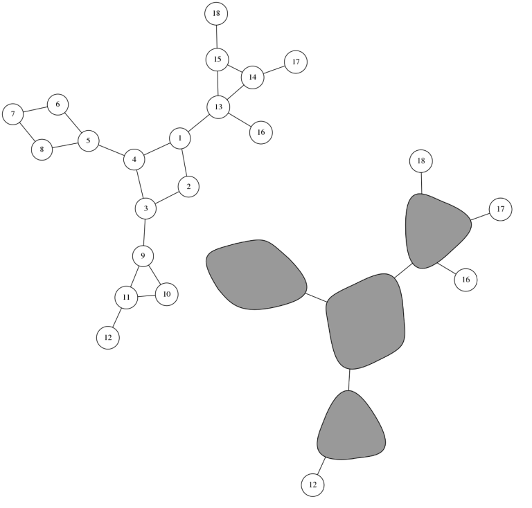
A cactus is a graph where every edge (or sometimes, vertex) belongs to at most one simple cycle. The first case is called an edge cactus, the second case is a vertex cactus. Cacti have a simpler structure than general graphs, as such it is easier to solve problems on them than on general graphs. But only on paper: cacti and cactus algorithms can be very annoying to implement if you don't think about what you are doing.
In the DFS tree of a cactus, for any span-edge, at most one back-edge passes over it. This puts cycles to an one-to-one correspondence with simple cycles:
- each back-edge forms a simple cycle together with the span-edges it passes over;
- there are no other simple cycles.
This captures most properties of cacti. Often, it is easy to implement cactus algorithms using this representation.
For example, consider this problem:
Problem 2. You are given a connected vertex cactus with $$$N$$$ vertices. Answer queries of the form "how many distinct simple paths exist from vertex $$$p$$$ to vertex $$$q$$$?".
This is named appropriately: 231E - Cactus. The official tutorial has a solution like this:
- "squeeze" every cycle to a single vertex, and paint these vertices black;
- root the tree;
- for each vertex $$$u$$$, calculate the number of black vertices on the path from the root to $$$u$$$; denote this $$$\mathrm{cnt}[u]$$$.
- the answer to query $$$(p, q)$$$ is either $$$2^{\mathrm{cnt}[p] + \mathrm{cnt}[q] - 2 \mathrm{cnt}[\mathrm{lca}(p, q)]}$$$ or $$$2^{\mathrm{cnt}[p] + \mathrm{cnt}[q] - 2 \mathrm{cnt}[\mathrm{lca}(p, q)] + 1}$$$ depending on the color of $$$\mathrm{lca}(p, q)$$$.
It isn't very hard to understand why this works. The more interesting part is implementation.

- "squeeze" every cycle to a single vertex, and paint these vertices black;
Great. How?
After some time, most people will probably find some way to implement this. But here is a simple way using the DFS tree:
- give each back-edge an unique index starting from $$$N + 1$$$;
- for each vertex $$$u$$$, calculate the index of the back-edge $$$u$$$ is under; call that $$$\mathrm{cycleId}[u]$$$; if $$$u$$$ isn't in a cycle then $$$\mathrm{cycleId}[u] = u$$$;
- form a new adjacency list where for each $$$u$$$, each instance of $$$u$$$ is replaced by $$$\mathrm{cycleId}[u]$$$.
Step 2 can be done like this, for example:
1  function visit(u):
2      for each vertex v among the children of u:
3          visit(v)
4
5      if there is a back-edge going up from u:
6          cycleId[u] = the index of that back-edge
7      else:
8          cycleId[u] = u
9          for each vertex v among the children of u:
10             if cycleId[v] != v and there is no back-edge going down from v:
11                 cycleId[u] = cycleId[v]
Removing edges to form a bipartite graph
Problem 3. Consider an undirected graph. Find all the edges whose removal will produce a bipartite graph.
This is 19E - Fairy. There is no official tutorial, but an unofficial tutorial mentions using complicated data structures like Link/cut tree. Using DFS tree, we can solve the problem without any advanced data structures.
In the original problem, the graph need not be connected. However, observe that:
- if the graph has no non-bipartite connected components, then removing any edge will produce a bipartite graph;
- if the graph has multiple non-bipartite connected components, then it is not possible to make the graph bipartite.
Thus, the only interesting case is when we have exactly one non-bipartite connected component. Obviously the edge we remove must also come from that component, so we can just pretend that this is the only component. From now on, we assume that we have a non-bipartite, connected graph.
Let's consider the DFS tree of the graph. We can paint the vertices black and white so that each span-edge connects a black vertex and a white vertex. Some back-edges, however, might connect two vertices of the same color. We will call these edges contradictory.
Observation 7. A back-edge $$$uv$$$ is a solution if and only if $$$uv$$$ is the only contradictory edge.
Observation 8. A span-edge $$$uv$$$ is a solution if and only if the set of back-edges passing over $$$uv$$$ is the set of contradictory edges.
Thus, we can solve the problem as such:
- find the DFS tree of the graph and paint it in two colors;
- if there is exactly one contradictory back-edge, add it to the answer;
- use dynamic programming to calculate, for each span-edge, how many contradictory and how many non-contradictory back-edges pass over it;
- if a span-edge has all contradictory and no non-contradictory edges passing over it, add it to the answer.
Directed variant
What happens if we find the DFS tree of a directed graph? Let's run our depth-first traversal again:
1 function visit(u):
2     mark u as visited
3     for each vertex v among the neighbours of u:
4         if v is not visited:
5             mark the edge u->v
6             call visit(v)
To clarify, on line 3 we only mean such vertices $$$v$$$ that there is an edge from $$$u$$$ to $$$v$$$.
It might be the case that this traversal never reaches some vertices. For simplicity, we assume that:
- we started the traversal at vertex 1, i.e. called
visit(1); - it is possible to reach every vertex from the vertex 1.
Let's call the edges marked at step 5 span-edges.
Observation 9. Span-edges form a rooted spanning tree, directed away from the root.
Other edges fall in two categories:
- edges that connect an ancestor with a descendant: back-edges;
- edges that don't: cross-edges.
It's possible to further divide the back-edges into up-edges and down-edges based on their direction.
Observation 10. Cross-edges are always directed from the vertex that was explored later, to the vertex that was explored earlier.
The directed variant of DFS tree is used to construct the dominator tree of a directed graph, but that is a beast on a whole another level that warrants its own tutorial.
Problems for practice
Solved in this tutorial:
Others:
- 858F - Wizard's Tour
- 412D - Giving Awards
- 101612G - Grand Test
- any task where you have to find a block-cut tree
If you know any other tasks that can be solved like this, share in the comment section! I might add them here, too.


