I have previously written about flows in these blogs: 1, 2, 3.

Minimum cuts are a very fascinating topic for me. There are a lot of maximum flow problems where there's a fairly simple chain of reductions leading to "you should use flow", but there are also a lot of flow problems where flow comes apparently out of nowhere. Particularly fascinating are those where it's more convenient to think in terms of minimum cut: they work, because minimum cut allows you to model partitioning a set in two, with some additional implication-like constraints. Here are a couple of problems with that nature:

• ARC085E - MUL (this reduction is almost standard these days)
• ARC142E - Pairing Wizards
• 104925D - Filesystem

There are also flow problems on graphs with special shapes where thinking in terms of cuts makes the flow easy to efficiently calculate.

• 724E - Goods transportation
• 1919F2 - Wine Factory (Hard Version)

Anyway, let's move on to the actual topic of the blog. I recently had a couple discussions on various Discord servers about some problems on minimum cuts. The problems were:

1. Given a flow network where all minimum cuts have a nonempty intersection, prove that there exists an edge that is in every minimum cut.
2. Given a flow network where each edge has a label (independent of capacity), calculate the lexicographically smallest minimum cut, in time $$$O(n^2 m)$$$.

Both problems involve statements like "among all minimum cuts". I thought the problems were very interesting, and shared a common thread, so I decided to write them up in a blog. They also lead neatly into some discussion of more general and abstract theory. $$$~$$$

Recap: maximum flow and minimum cut

I'm assuming that you are already familiar with flows and cuts, so this will be brief, just so we are all on the same page.

Given a directed graph $$$G = (V, E)$$$ with two special vertices $$$s$$$ and $$$t$$$ ("source" and "sink"), the maximum flow problem asks you to assign to each edge a flow $$$f_e$$$, which is either 0 or 1, such that for every vertex except $$$s$$$ and $$$t$$$, the amount of incoming flow equals the amount of outgoing flow. You need to maximize the amount of outgoing flow from $$$s$$$ (minus the amount of incoming flow to $$$s$$$).

Given a directed graph $$$G = (V, E)$$$ with two special vertices $$$s$$$ and $$$t$$$, the minimum cut problem asks you to partition the set of vertices in two: $$$X$$$ and $$$V \setminus X$$$, such that $$$s \in X$$$, $$$t \notin X$$$ and the number of edges directed from $$$X$$$ to $$$V \setminus X$$$ is minimized. (There are no constraints for edges from $$$V \setminus X$$$ to $$$X$$$.) I'll refer to both the set $$$X$$$ and the set $$$\delta^+(X)$$$ — the set of edges leaving $$$X$$$ — as a "(minimum) cut". It should be clear from the context which is meant.

For the purposes of this blog, I'll only consider the case with unit capacities. This is not a serious loss of generality: if an edge has capacity $$$c$$$ for a positive integer $$$c$$$, you can replace this edge with $$$c$$$ identical edges. If some edges have fractional capacities, you can first multiply all capacities by their lowest common denominator, then do the thing above. After getting the answer, divide it by the lowest common denominator. I'll not consider the case where capacities can even be irrational. Therefore, anything I prove about flow networks with unit capacities is also true for flow networks with rational capacities, and in implementations you can still do the normal thing without any slowdown.

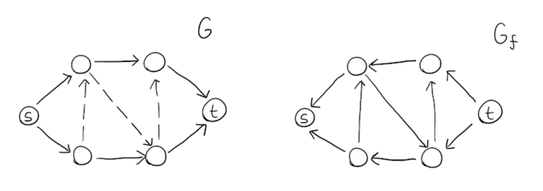
Also important to us is the concept of the residual graph. Given a flow $$$f$$$ on $$$G$$$, not necessarily maximum, the residual graph $$$G_f$$$ is obtained by taking $$$f$$$ and reversing all edges that have flow on them. In this blog, pay close attention to whether an edge is in $$$G$$$ or $$$G_f$$$.

The relationship between maximum flow and minimum cut

The maximum flow and minimum cut problems have the exact same type of input data. You might be aware that the numerical answer is also the same. Do you know why?

Observation. The maximum flow is at most the minimum cut.

Observation. There is a cut with value exactly that of the maximum flow.

This is all pretty well-known, but did you know that the relationship goes deeper than that? And even without any real extra work to prove it!

Observation. Let $$$f$$$ be any maximum flow. A set of vertices $$$X$$$ with $$$s \in X, t \notin X$$$ forms a minimum cut if and only if in the residual graph $$$G_f$$$, there are no edges directed from $$$X$$$ to $$$V \setminus X$$$.

This observation gives us a nice characterization of the set of all minimum cuts, and a technique for solving problems like "is there a minimum cut such that ..." or "find a minimum cut such that ...": take any maximum flow $$$f$$$, find the residual graph $$$G_f$$$ and work with that.

Problem 1: intersections of minimum cuts

Problem. Given a flow network where all minimum cuts have a nonempty intersection, prove that there exists an edge that is in every minimum cut. The intersections are taken edge-wise.

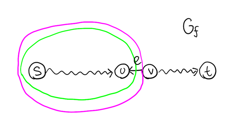
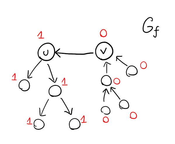
What previously seemed like an impossible task becomes easy now. Let $$$f$$$ be any maximum flow and $$$G_f$$$ its corresponding residual graph. There are two things that must hold for any minimum cut $$$X$$$:

• Every vertex reachable from $$$s$$$ in $$$G_f$$$ is definitely $$$X$$$.
• Every vertex from which $$$t$$$ is reachable in $$$G_f$$$ is definitely not in $$$X$$$.

In fact, this also gives us two minimum cuts (which might be equal) straight away:

• A cut that consists exactly of the vertices reachable from $$$s$$$ in $$$G_f$$$.
• A cut that consists of all vertices except those from which $$$t$$$ is reachable in $$$G_f$$$.

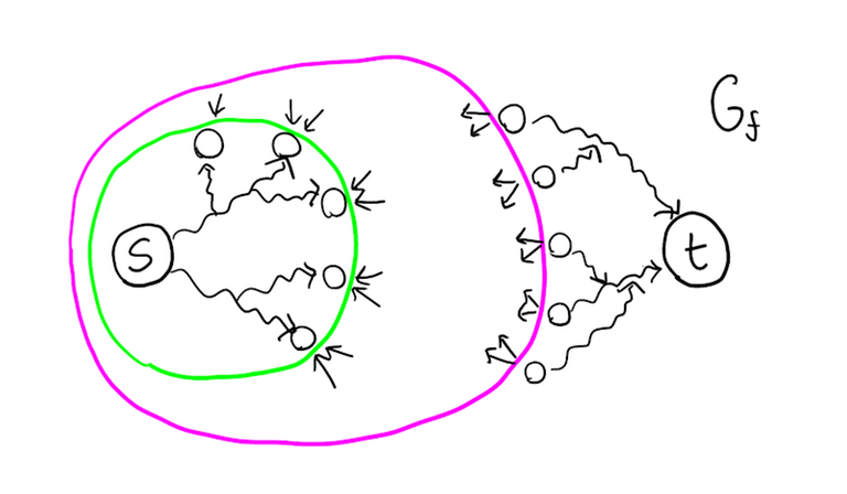
If these two cuts have no common edges, then we are done. Otherwise, there exists some edge $$$u \to v$$$ in $$$G$$$ such that there exist paths $$$s \leadsto u$$$ and $$$v \leadsto t$$$ in $$$G_f$$$. But that means that $$$u$$$ is in all minimum cuts and $$$v$$$ is in no minimum cuts, which means that $$$u \to v$$$ is in every minimum cut and we are again done.

Problem 2: lexicographically smallest minimum cut

Problem. Given a flow network where each edge has a label (independent of capacity), calculate the lexicographically smallest minimum cut, in time $$$O(n^2 m)$$$. Minimum cuts are compared lexicographically edge-wise, i.e. each cut is a list of edge labels.

The specific time complexity is actually not so important: the point is that the running time of the algorithm should be dominated by $$$O(1)$$$ calls to a maximum flow algorithm, say Dinitz's algorithm.

Whenever we are asked to find the lexicographically smallest sequence subject to some constraints, the general structure of the algorithm is almost always the same. Start building the sequence; for each prefix check if there are any solutions with that prefix. If there aren't, replace the last element of the prefix with the next smallest thing. The same applies in this problem.

• Set $$$C = \varnothing$$$. (The set of the edges in the cut)
• For each edge $$$e$$$, in increasing order of label:
• • Check if there exists a minimum cut that contains all edges in $$$C \cup \{ e \}$$$.
• • If there does, add $$$e$$$ to $$$C$$$.

Let $$$f$$$ be any maximum flow and $$$G_f$$$ the residual graph. To check if there exists a minimum cut containing all edges in $$$C$$$, we need to check if we can assign 0 or 1 to each vertex such that:

• For each edge $$$u \to v$$$ in $$$C$$$, $$$u$$$ must be assigned 1 and $$$v$$$ must be assigned 0.
• $$$s$$$ must be assigned 1.
• $$$t$$$ must be assigned 0.
• If any vertex $$$u$$$ is assigned 1, and there's an edge $$$u \to v$$$ in $$$G_f$$$, then $$$v$$$ must also be assigned 1.
• If any vertex $$$v$$$ is assigned 0, and there's an edge $$$u \to v$$$ in $$$G_f$$$, then $$$u$$$ must also be assigned 0.

We can check this with DFS: set 0 to everything that must be assigned 0 and 1 to everything that must be assigned 1. Use DFS to "propagate" the 1-s over forward-edges and the 0-s over backward-edges. If at any point there's a contradiction (a vertex must be assigned both 0 and 1) then the answer is "no". Otherwise, the answer is yes. If implemented carefully, this takes $$$O(m + n)$$$ time.

This is pretty good — we only need to calculate the maximum flow once — but we still need to do a full scan for each edge, taking $$$O(m (m + n))$$$ time. Instead of recalculating everything for each edge we try to add to the cut, we should do the work incrementally:

• Set $$$C = \varnothing$$$.
• Assign an "indeterminate" value to each vertex.
• Assign 1 to $$$s$$$, do a DFS to assign everything reachable from $$$s$$$ in $$$G_f$$$ also 1.
• Assign 0 to $$$t$$$, do a DFS to assign everything $$$t$$$ is reachable from in $$$G_f$$$ also 0.
• For each edge $$$e = u \to v$$$ of $$$G$$$ in increasing order of label:
• • Assign 1 to $$$u$$$, do a DFS to assign everything reachable from $$$u$$$ in $$$G_f$$$ also 1.
• • Assign 0 to $$$v$$$, do a DFS to assign everything $$$v$$$ is reachable from in $$$G_f$$$ also 0.
• • If there was a contradiction in either of the above, roll-back all changes made in this step.
• • Otherwise, add $$$e$$$ to $$$C$$$.

If there were no rollbacks, this takes $$$O(n + m)$$$ time (you should write DFS so that it never sets the same value to the same vertex multiple times). But the rollbacks can make this expensive, so we need a way to quickly check whether trying to add $$$u \to v$$$ of $$$G$$$ would cause a contradiction. It turns out that this can only happen if either $$$u$$$ or $$$v$$$ already has the wrong value assigned or if there is a path $$$u \leadsto v$$$ in $$$G_f$$$, which in turn only happens if $$$u \to v$$$ in $$$G$$$ is oriented $$$u \to v$$$ in $$$G_f$$$ or if $$$u$$$ and $$$v$$$ are in the same strongly connected component in $$$G_f$$$.

Generalizing this relationship: complementary slackness

We've now discovered that that the relationship between maximum flow and minimum cut is incredibly powerful: they are not merely equal by happenstance, but deeply intertwined. Knowing one maximum flow allows us to characterize the set of all minimum cuts.

This is a general phenomenon, not limited to just flows and cuts. It's called duality, and the idea that one maximum flow can be used to check any cut for minimality has a fancy name too: complementary slackness. Let's write down the definition of a maximum flow in terms of equalities and inequalities.

Here, $$$\delta^+ (v)$$$ refers to the set of all outgoing edges from $$$v$$$, and $$$\delta^- (v)$$$ refers to the set of all incoming edges to $$$v$$$. Note that this system of (in)equalities allows $$$f_e$$$ to be anything between 0 and 1, but this is not actually a different problem: there will always be at least one maximum solution consisting of only integers.

Systems of linear equalities and inequalities like this are called linear programs. Every linear program has a dual program, constructed as follows.

• The dual program has a variable for every constraint in the primal program, and a constraint for every variable in the primal program.
• The coefficients are obtained by transposing, i.e. the coefficient of the $$$i$$$-th variable in the $$$j$$$-th constraint becomes the coefficient of the $$$j$$$-th variable in the $$$i$$$-th constraint.
• In the objective function, minimization becomes maximization and vice versa.
• The coefficients of the objective function become the right-hand sides in the constraints, i.e. the coefficient of the $$$i$$$-th variable in the objective function becomes the right-hand side of the $$$i$$$-th constraint.
• The right-hand sides in the constraints become the coefficients in the objective in the same way.
• Whether a constraint in the dual is $$$\le$$$, $$$\ge$$$ or $$$=$$$ depends on whether the corresponding variable was nonnegative, nonpositive or free, using the following table.

The dual linear program for maximum flow is exactly that of minimum cut:

Let's convince ourselves that the optimum is indeed minimum cut. We have to set a value $$$x_u$$$ to each vertex. Obviously, since we want to minimize the sum of $$$y_e$$$-s, it is always optimal to set $$$y_e = \max(0, x_u - x_v)$$$.

Suppose we have a set $$$X$$$ such that $$$s \in X$$$ and $$$t \notin X$$$. Set $$$x_u = 1$$$ for $$$u \in X$$$ and $$$x_u = 0$$$ for others. Then, if we set $$$y_e = \max(0, x_u - x_v)$$$, we have that $$$y_e = 1$$$ if and only if $$$e$$$ is an edge from $$$X$$$ to $$$V \setminus X$$$. Thus the objective function simply counts the number of cut edges. Therefore, if this linear program has at least one optimal solution with $$$x_u \in \{0, 1\}$$$, then the set of minimum cuts is precisely the set of optimal solutions to this linear program that have $$$x_u \in \{0, 1\}$$$.

There are two very important facts about duality.

Theorem ("strong duality"). Assuming both the primal and the dual linear program are feasible, their optimal objective values are equal.

"Feasible" means that that there is at least one solution. There are also linear programs with no solutions (e.g. maximize $$$x$$$ subject to $$$x \le 0$$$ and $$$x \ge 1$$$). These are not relevant here, so I'll not discuss them for the time being.

Now we know that the dual linear program has at least one optimal solution with $$$x_u \in \{0, 1\}$$$: take any maximum flow, its value is equal to any minimum cut, and this minimum cut minimizes the objective value — the optimal value for the dual can't be less than the value of the maximum flow as that would violate strong duality. Therefore, the set of minimum cuts is precisely the set of optimal solutions to this linear program that have $$$x_u \in \{0, 1\}$$$.

Now comes the second very important fact about duality.

Theorem ("complementary slackness"). Let $$$f$$$ be a feasible solution of the primal program and $$$(x, y)$$$ a feasible solution of the dual program. They are both optimal if and only if the following hold:

• For every nonfree variable in the primal problem, the variable is 0 or equality holds in the corresponding dual constraint.
• For every nonfree variable in the dual problem, the variable is 0 or equality holds in the corresponding primal constraint.

In case of max-flow/min-cut, this means that a feasible $$$f$$$ and a feasible $$$(x, y)$$$ are both optimal if and only if:

• For every edge $$$e$$$, $$$f_e = 0$$$ or $$$x_u - x_v = y_e$$$.
• For every edge $$$e$$$, $$$f_e = 1$$$ or $$$y_e = 0$$$.

If we already know that $$$f$$$ a maximum flow, we can use it to check whether some given $$$X$$$ constitutes a minimum cut. Take a $$$X$$$, set $$$x_u = 1$$$ for $$$u \in X$$$ and $$$x_u = 0$$$ for others. Set $$$y_e = \max(0, x_u - x_v)$$$. Notice that only the following ban $$$X$$$ from making a minimum cut:

• $$$f_e > 0$$$ and $$$x_u - x_v < y_e$$$, which can only happen if $$$f_e = 1$$$, $$$x_u = 0$$$, $$$x_v = 1$$$.
• $$$f_e < 1$$$ and $$$y_e > 0$$$, which can only happen if $$$f_e = 0$$$, $$$x_u = 1$$$, $$$x_v = 0$$$.

Therefore, a set $$$X$$$ makes a minimum cut if and only if there are no edges from $$$V \setminus X$$$ to $$$X$$$ with flow on them, and no edges from $$$X$$$ to $$$V \setminus X$$$ with no flow on them. Or in terms of the residual graph, if and only if there are no edges from $$$X$$$ to $$$V \setminus X$$$ in the residual graph. This is precisely the condition we saw earlier.

Although such general duality is a somewhat more theoretical concept, it can be useful to think about competitive programming problems. See for example:

• UCup season 1 stage 10: H - Hard Problem
• WTF 2022 day 1: D - Welcome to Tokyo!