


I once read a paper that claimed and used the fact that the Hungarian algorithm can be implemented in such a way that it runs in $$$O(m n \log n)$$$ time. Using the soft-O notation which ignores log factors, the complexity can be written as $$$\tilde{O} (m n)$$$. If the graph is dense, i.e. $$$m = \Theta(n^2)$$$, the log factor can be removed There are many tutorials on how to get $$$O(n^3)$$$, but I couldn't find any references that directly show how to do $$$\tilde{O}(mn)$$$ from end to end (but I found just enough to conclude that it is probably possible). So I decided to write one up myself and well, this is as good a place as any.
In my last blog, I showed how thinking in terms of linear programming and duality can be useful when working with maximum flows and minimum cuts. The usefulness of this is best demonstrated with examples, and this is a good example. In fact, this is pretty much the primal-dual algorithm: it was one of the prototypes that inspired the entire theory. So, this should in fact be an excellent example to gain more intuition of the concept.
As I said, this algorithm makes a nice case study of linear programming and duality. It also brings together many other ideas, so this is a learning opportunity for many things.
Problem statement
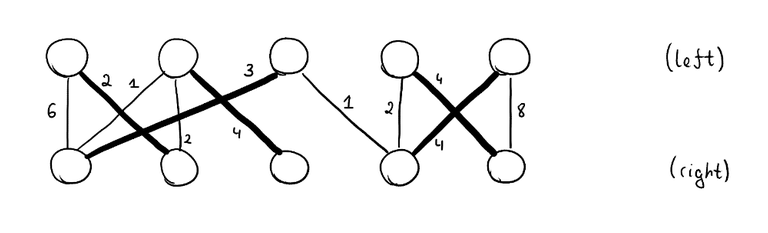
You are given a bipartite graph with $$$n$$$ vertices and $$$m$$$ edges. Each edge has a cost $$$c_e$$$. You want to find the minimum cost perfect matching: each vertex on the left must be matched to exactly one vertex in the right and vice versa. The sum of the costs of the edges that are in the matching must be minimized. We assume that at least one perfect matching always exists.
 $$$~$$$
The linear programming formulation and its dual
This time I'll go with linear programming from the start.
For each edge, we make a variable $$$x_e$$$, which should be 1 if the edge is in the matching and 0 if it isn't. We have a perfect matching if and only if each vertex is incident to exactly one edge in the matching. Thus, we seek to find a solution to the following problem.
The last constraint, $$$x_e \in \{0, 1\}$$$, is very annoying to work with, and in general, such constraints are fundamentally very hard to satisfy. Thus, we replace $$$x \in \{0, 1\}$$$ with $$$0 \le x \le 1$$$. After adding a $$$x_e \ge 0$$$ constraint for each edge, an $$$x_e \le 1$$$ constraint would actually be redundant: the sum of $$$x_e$$$-s incident to any vertex must be 1, and they are all nonnegative, so there's no way $$$x_e$$$ could ever be greater than 1 anyway.
This is not actually a different problem: it can be shown that there will always exist at least one minimizer where all $$$x_e$$$ are integer.
The dual of this linear program is
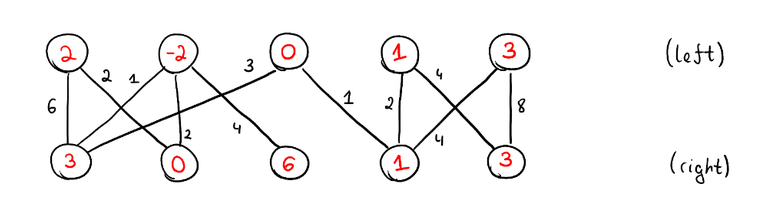
We have to assign to each vertex a value $$$y_v$$$. We call these values potentials, they are also sometimes called prices. We need to do it in such a way that for each edge, the sum of potentials on its endpoints does not exceed the cost of the edge, but the total sum of potentials is as high as possible. It can be shown that as long as the $$$c_e$$$ are integers, there will always be at least one optimal solution where $$$y_v$$$ are all integers too.
As you can see, the potentials may very well be negative. Recall the two important theorems about duality:
Theorem ("strong duality"). Assuming both the primal and the dual linear program are feasible, their optimal objective values are equal.
Theorem ("complementary slackness"). Let $$$x$$$ be a feasible solution to the primal problem and $$$y$$$ a feasible solution to the dual problem. They are both optimal if and only if the only if the following hold:
- For every nonfree variable in the primal problem, the variable is 0 or equality holds in the corresponding dual constraint.
- For every nonfree variable in the dual problem, the variable is 0 or equality holds in the corresponding primal constraint.
What does this mean in our situation? There are no nonfree variables in the dual problem, so this theorem only states that $$$x$$$ and $$$y$$$ are both optimal if and only if for each edge $$$e$$$, $$$x_e = 0$$$ or $$$y_u + y_v = c_e$$$. In other words, given a matching $$$x$$$ and potentials $$$y$$$, both are optimal if and only if the matching only uses edges where $$$y_u + y_v = c_e$$$.
We'll call such edges tight (they are also sometimes called rigid). Since we want to maximize the sum of $$$y_v$$$-s, we'd generally like to set $$$y_v$$$-s to values as high as possible. Tight edges are the ones where the potential of one endpoint cannot be increased without decreasing the other one at least as much. Restated slightly, the complementary slackness condition now reads:
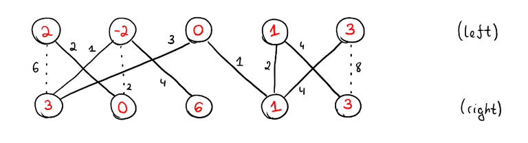
Corollary. A dual solution $$$y$$$ is optimal if and only if there exists a perfect matching that only uses the tight edges of $$$y$$$. That matching is a solution to the primal problem.
Looking at the dual solution above, it's hard to understand whether it's optimal or not. With this corollary it becomes clear. Yes, because there's a perfect matching using only the tight edges. Here and in future images, non-tight edges are represented as dotted edges.
The way this property just falls out is why duality and complementary slackness are useful. I could prove this property from scratch, and many tutorials do, but why? It's just going to be annoying set-theoretic casework. This is why abstractions are useful. They remove repeated work. We have seen the same kinds of arguments many times. Why go through this reasoning every time? It's the same reason why you call std::sort in your code: it makes no sense to write the same logic every time. It's much better to extract the logic that actually differs between problems and pass that in as a comparator. The only difference here is that in this case, the abstraction is a lot less obvious: it's much harder to see that properties of this type are special cases of the same thing.
The basic Hungarian algorithm
Now, let's think about how we'd actually solve the minimum cost perfect matching problem. Because of strong duality, we know that we can solve the dual problem instead. The last corollary is really powerful because it gives us a way to check a given $$$y$$$ for optimality: simply run a regular matching algorithm on a graph that consists only of the tight edges. This means that we could imagine an algorithm that looks like this (this is just a rough template, in reality the steps will be somewhat more intertwined):
- Set $$$y$$$ to be some feasible solution, say $$$y_v = 0$$$ for all vertices $$$v$$$ (or $$$y_v = -\infty$$$ if costs can be negative).
- Loop:
-
- Find the maximum matching $$$M$$$ on the graph formed of only the tight edges.
-
- If $$$M$$$ is perfect, break out of the loop: $$$y$$$ is a solution.
-
- "Improve" $$$y$$$ somehow.
The complementary slackness is really important here: if we didn't have an optimality condition like this, we would not know when to stop improving it. But now, we only need to come up with a system to improve $$$y$$$ and prove that it keeps making progress.
Improving $$$y$$$
We have assigned each vertex a potential and calculated a maximum matching $$$M$$$ on the edges that are tight. We have found that this maximum matching is not a perfect matching. Now we are tasked with improving $$$y$$$. There are no constraints on how exactly this must be done, except that $$$y$$$ must remain a valid feasible solution afterwards. These "improvements" should also make progress in some sense: later we need to prove that after a fixed number of iterations, we have found an optimal solution.
It seems natural to try improving $$$y$$$ in a way that increases the objective function — afterwards, the sum of all potentials should be higher than before. It turns out that we can actually use the fact that there is no perfect matching on this subgraph of tight edges.
Theorem (Hall's marriage theorem). A bipartite graph with $$$n$$$ vertices on both sides has a perfect matching if and only if for every subset $$$S$$$ of vertices on the left side, $$$\left| N(S) \right| \ge \left| S \right|$$$. Here, $$$N(S)$$$ is the set of vertices on the right side that have an edge to one of the vertices of $$$S$$$.
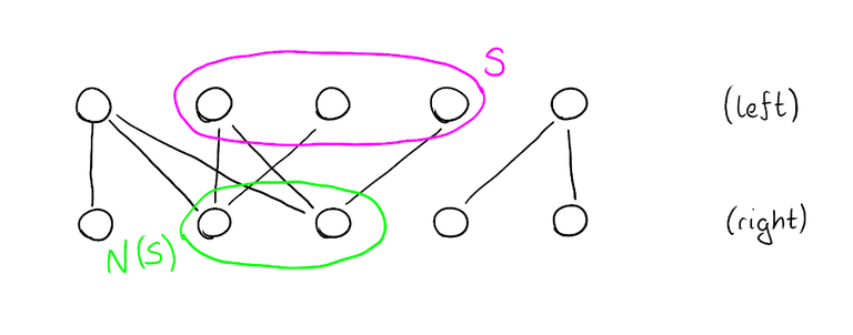
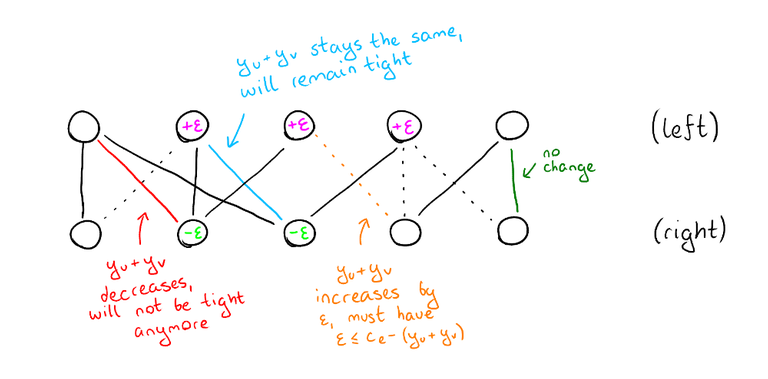
Since we know that the tight subgraph doesn't have a perfect matching, we know that there must be at least one set of vertices $$$S$$$ on the left side such that $$$\left| N(S) \right| \lt \left| S \right|$$$. Let's find a set $$$S$$$ like that, and increase the potential of all vertices in $$$S$$$ by some small $$$\varepsilon \gt 0$$$, and decrease the potential of all vertices in $$$N(S)$$$ by $$$\varepsilon$$$. Denote these new potentials by $$$y'$$$. This operation increases the total sum of potentials because there are more vertices where we increased the potential than there are vertices where we decreased the potential.
But is $$$y'$$$ also feasible? We need to check that $$$y'_u + y'_v \le c_e$$$ for all edges $$$e = uv$$$. There are four cases:
- $$$u \in S, v \in N(S)$$$. Then $$$y'_u + y'_v = y_u + \varepsilon + y_v - \varepsilon = y_u + y_v \le c_e$$$.
- $$$u \in S, v \notin N(S)$$$. Then $$$y'_u + y'_v = y_u + y_v + \varepsilon$$$. But we know that these edges are not tight, otherwise $$$v$$$ would be in $$$N(S)$$$. Thus $$$y_u + y_v \lt c_e$$$, which means that for a small enough $$$\varepsilon$$$, $$$y'_u + y'_v \le c_e$$$ still.
- $$$u \notin S, v \in N(S)$$$. Then $$$y'_u + y'_v = y_u + y_v - \varepsilon \lt y_u + y_v \le c_e$$$.
- $$$u \notin S, v \notin N(S)$$$. Then $$$y'_u + y'_v = y_u + y_v \le c_e$$$.
So, $$$y'$$$ is feasible as long as we pick a small enough $$$\varepsilon$$$ and has a higher sum of potentials than $$$y$$$. But that is not enough to show that the algorithm actually terminates or even converges. Maybe after the first iteration we have sum of potentials $$$1$$$, after the second $$$1.5$$$, after the third $$$1.75$$$ and so on, but the real optimum is $$$400$$$?
That is not the case, if we always use the highest $$$\varepsilon$$$ we can. If $$$c_e$$$ are all integers, this means that we can always at least choose $$$\varepsilon = 1$$$ and thus increase the sum of potentials by at least 1 every time. But in fact, we can do much better. We'll return to this after the next section.
Finding a Hall violator
Now we know how to improve the sum of potentials if we have a set $$$S$$$ of vertices on the left side such that $$$\left| S \right| \gt \left| N(S) \right|$$$. Therefore, we need a reasonably fast algorithm to actually calculate that.
We want to find a set $$$S$$$ and a set $$$N(S) = T$$$. Let's fix an unmatched vertex $$$r$$$ and decide that $$$r$$$ must be in $$$S$$$. We make two additional rules:
- If $$$u$$$ is in $$$S$$$, then all of its neighbors must be in $$$T$$$ (which follows from $$$N(S) = T$$$ anyway).
- If $$$u$$$ is in $$$T$$$, the vertex it is matched with must be in $$$S$$$.
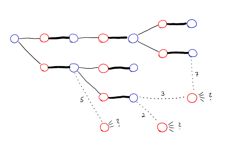
We can easily do this with DFS. But why are these rules helpful? The tree of vertices explored by DFS looks like this:
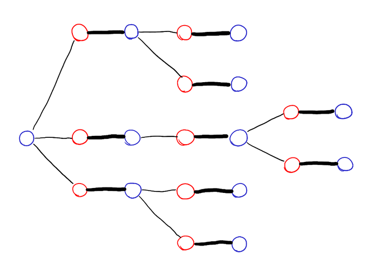
The vertices on the left side are bLue, the vertices on the right side are Red. I claim that all leaves of this tree are on the left side. Indeed, suppose there were leaves on the right side, take the one that was first explored, call it $$$u$$$. It must be unmatched — it can't be matched to any previously explored vertex, because all previously explored vertices except $$$r$$$ are matched, and their neighbor in the matching is their parent or child. But then, it means that there is a path from $$$r$$$ to $$$u$$$ like this:
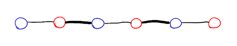
But that means that the matching isn't actually maximum, because we can find a bigger one by inverting the path:
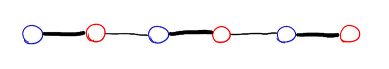
Therefore, $$$S$$$ has one more vertex than $$$T$$$, which is exactly what we wanted. Clearly, we can calculate $$$S$$$ in $$$O(n + m)$$$ time. Also, the DFS is actually irrelevant. We are simply calculating the set of vertices reachable from $$$r$$$ in a directed graph formed taking all the tight edges, directing the edges of the matching from right to left and all others from left to right.
Why improving $$$y$$$ makes progress and the $$$O(n^2 m)$$$/$$$O(n^4)$$$ version of the algorithm
Once we have found a Hall-violator $$$S$$$, we increase the potential of the vertices in $$$S$$$ by some $$$\varepsilon$$$ and decrease the potential of the vertices in $$$N(S)$$$ by the same $$$\varepsilon$$$. We choose the largest $$$\epsilon$$$ such that $$$y$$$ remains a valid potential, that is,
i.e. the smallest value of $$$c_e - (y_u + y_v)$$$ among edges $$$e = uv$$$ that are not tight, such that $$$u \in S$$$ and $$$v \notin S$$$. After this change, the edge $$$e = uv$$$ becomes tight. As a result, one of two things will happen:
- The size of the maximum matching in the tight subgraph changes. Since the edges of the old maximum matching are still tight, it means that the maximum matching must have become larger.
- The number of reachable vertices from $$$r$$$ (using the rules above) becomes bigger, since we are now obligated to include $$$v$$$.
This means that the algorithm now looks like this:
The outer loop has $$$O(n)$$$ iterations because the maximum matching increases by at least 1 every time, and the inner loop has $$$O(n)$$$ iterations because the number of reachable vertices increases by at least 1 every time.
Up until now, we have assumed that the maximum matching is calculated by some black-box maximum matching algorithm. But this doesn't make much sense, because it's potentially expensive to recalculate the maximum matching from scratch every time. And our DFS can already handle that: if we discover a leaf on the right side, we know how to increase the size of the maximum matching. Thus:
By the same reasoning as above, the loop has $$$O(n^2)$$$ iterations. Every operation in the loop can be done in $$$O(n + m)$$$ time, which gives $$$O(n^2 m)$$$ for sparse graphs and $$$O(n^4)$$$ for dense.
Optimization to $$$\tilde{O} (n m)$$$ or $$$O(n^3)$$$
Take a look at the algorithm above. There is one glaring inefficiency. In every iteration of the loop, we do the entire DFS from scratch, even if the matching hasn't changed. Why? There are some new edges, sure, but the tree remains the same for the previously explored vertices. We should add to the tree, not rebuild it. So, when you are doing DFS and looking at the edges exiting a blue vertex, also look at the edges that are not tight. For each of them, calculate the maximum amount the potentials on the endpoints can be increased before this edge becomes tight. Push those values in a priority queue.
Next time you would do DFS, keep the previously explored tree intact and take the edge with the smallest value from that priority queue. If the other endpoint is already explored, ignore it, otherwise explore from there.
Care must be taken to update the vertex potentials correctly. Don't update them every time; instead note the $$$\varepsilon$$$ used in each step, and for each vertex the step during which it was explored. The adjusted vertex potential will at the end be the corresponding suffix sum. Similarly, after each step, you should reduce each key in the priority queue by $$$\varepsilon$$$. This can be simulated by instead adding $$$\varepsilon$$$ to each subsequently pushed element to the priority queue.
What is the complexity now? The maximum matching can increase only $$$O(n)$$$ times. For each size of the maximum matching, we do a sequence of DFS-s that in total explore every edge at most once, so the DFS part has complexity $$$O(n + m)$$$. We also need to find the edge with the smallest key, that happens $$$O(m)$$$ times. Each push and pop to the priority queue takes $$$O(\log m) = O(\log n)$$$ time, which means $$$O(n (n + m + m \log n)) = O(m n \log n)$$$.
If the graph is dense, we can replace the priority queue with an array that for each unexplored vertex contains the edge with the smallest slack. We need to $$$O(n)$$$ times find the least element of this array, which can done by iterating in $$$O(n)$$$. The DFS now takes in total $$$O(n^2)$$$, which gives $$$O(n^3)$$$ in total.
Exercise
In this blog, we considered the case where the left and right sides are equal. Try to convert everything to the case where there are fewer vertices on the left than on the right. Instead of "perfect", we now want "everything on the left side is matched".


Isn’t running $$$n$$$ iterations of Dijkstra yielding $$$O(n m \log m)$$$ complexity? I always thought these ‘primal-dual’ Hungarian algorithms are more or less optimizations of SSPA on the special structure of the graph, are they not?
I think so, yes.
SSPA is also primal-dual, actually. The vertex potentials you use to make the edge costs nonnegative can be analyzed as a dual (I believe adamant has written about that). Since min-cost flow is a generalization of min-cost matching, it makes sense that if you take the "natural" primal-dual algorithm for min-cost flow, restrict it to the matching case and simplify, you'll get something very similar to the "natural" primal-dual algorithm for min-cost matching, i.e. the above. Though it's unfortunate that this doesn't result in an asymptotic speedup.
Yeah, that was my point as well. There might however be some differences, as Hungarian is incremental (you can add, and maybe also remove? vertices in $$$O(m \log m)$$$), which I believe isn’t possible, or at least not in a straightforward way, with SSPA.
Thank you!
You formulated a linear programming problem (and then solved its dual). Do you understand what happens if we try to solve any of the primal/dual using, for example, the simplex algorithm? Can it happen that it will do exactly the same as we do with arbitrary pivot rule? Because increasing something and decreasing something else while something holds looks an awful lot like moving along an edge of a polytope until we reach another vertex. If that turns out to be the case, it will add another layer of abstraction, which is nice for understanding the structure.
Thank you for the great tutorial; now I understand the Hungarian algorithm.
I think it has a lot of applications, particularly in combinatorial optimization.
This problem can be solved using Hungarian algorithm.
Problem: 1354F - Призыв существ