Each edge on the tree is classified into 2 types: heavy and light.

Let treeSize[u] = the number of nodes in the subtree rooted at node u.

Consider any node u with children v1, v2, ..., vk → we have edges (u, v1), (u, v2), ..., (u, vk).

Among these children, let vi be the child with the largest treeSize (if multiple children have the same largest treeSize, we can pick any one of them).

Then, the edge (u, vi) is called a heavy edge.

The remaining edges are light edges.

Basic properties:

For every node u (except the root), there is exactly one heavy edge going from u to one of its children.

If the edge (u, vi) is a light edge, then we have: treeSize[u] > 2 * treeSize[vi]

Proof of property (2):

Assume (u, vi) is a light edge → there exists another child vj of u (vj ≠ vi) such that edge (u, vj) is the heavy edge.

By the rule of selecting the heavy edge, vj is the child with the largest treeSize.

This means: treeSize[vi] ≤ treeSize[vj].

On the other hand, the subtrees rooted at vi and vj are disjoint (since they belong to different branches of the subtree rooted at u), so:

treeSize[vi] + treeSize[vj] < treeSize[u].

From this, we derive: treeSize[u] > 2 * treeSize[vi].

Advanced Consequences: (A) Since no two heavy edges share the same parent, heavy edges form chains. (B) On any path from an arbitrary node x to the root, the number of light edges is at most log(n).

For each light edge, we have treeSize[parent] > 2 * treeSize[child].

This means that every time we move upward through a light edge, the subtree size at least doubles. Since treeSize[root] = n, the number of times we can double before reaching the root is at most log(n).

→ Therefore, on the path between any two nodes (u, v), the number of light edges is at most 2 * log(n).

To list all heavy-edge chains simply, we perform a DFS on the tree.

During DFS, we always explore the heavy child first before visiting other branches.

This way, all nodes in the same heavy-edge chain will be visited consecutively.

The following image shows the original tree structure before applying heavy-light decomposition.

At this stage, all edges are considered equal, and no heavy paths have been identified yet.

Now, after applying the heavy-light decomposition, the tree is broken into several heavy-edge chains.

Heavy edges (typically shown in bold or color) form continuous paths that optimize traversal and queries.

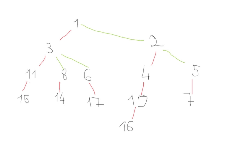
The sequence below shows the order in which nodes are visited during a depth-first search (DFS) traversal.

1 → 3 → 11 → 13 → 15 → 12 → 8 → 14 → 17 → 6 → 2 → 4 → 10 → 16 → 9 → 5 → 7

Heavy-Light Decomposition is a powerful technique to break down a tree into heavy and light edges, helping optimize many tree-related problems. This introduction covered the basic concepts and how to identify heavy edges using DFS.

In the next post, we will dive deeper into how to implement HLD efficiently and apply it to solve practical problems.

Stay tuned!